Show the code
## the whittakerr toolkit
library(whittakerr)
## read_csv() for the inline cities table
library(readr)
## suppress read_csv() column-type messages
options(readr.show_col_types = FALSE)Every boundary this document has drawn has been a clean line. The polygon edges of the Whittaker diagram, the sharp color borders of the biome map: a biome ends, and the next begins, at a definite place. That clean line is a convenience. It is also, like every useful simplification, not quite true.
A real biome boundary is a zone, not a line, and it takes two forms. Across space it is the ecotone, the band of country where two biomes meet and intergrade rather than abut. Across time it is the climate shift, a place’s climate moving through temperature-precipitation space and, sometimes, across a boundary the diagram draws. This chapter follows both. The edges, it turns out, in space and in time alike, are where the most is at stake.
## the whittakerr toolkit
library(whittakerr)
## read_csv() for the inline cities table
library(readr)
## suppress read_csv() column-type messages
options(readr.show_col_types = FALSE)On the diagram, the boundary between two biomes is a polygon edge, a line with no width. On the ground it is nothing of the kind. Travel from forest into grassland and there is no line to cross. There is a band, often tens of kilometers wide, where the forest thins, the trees draw apart, grass opens between them, and one biome gives way to the other. That band is the ecotone.
The ecotone is not empty transitional ground. It is, characteristically, the richest ground. A site within it can hold species from the forest, species from the grassland, and species that belong to the edge itself, to conditions that exist only where the two biomes meet. Ecologists have a name for the pattern, the edge effect: diversity tends to peak not in the interior of a biome but along its margins. The boundary the diagram draws as a thin line is, in the field, the place with the most life in it.
This is the first sense in which the crisp boundary is a simplification. The diagram has to draw a line, because a polygon needs an edge, and the line is not wrong: it marks where the balance tips from one biome to the other. But the line stands for a zone. A climate point that sits close to a polygon edge is a site in or near an ecotone, and the Retrieving Biome Information chapter’s closing question, how far a point lies from a boundary, is in the field a question about how deep into an ecotone a site sits.
The boundary’s second form is harder to see, because it moves. A place’s climate is not fixed. Over decades, under a changing climate, a location’s annual temperature and precipitation drift, which is to say the point representing it drifts through the Whittaker diagram. If it drifts far enough, it crosses a polygon edge, and the place is projected to belong to a different biome than the one it belongs to now.
The toolkit can show this directly. map_biomes() builds a region’s biome map from climate data, and it accepts a future climate as readily as a historical one: with scenario = "future" it draws on a CMIP6 projection in place of the 1970-2000 baseline. Map a region twice, once as it is and once as a projection has it, and the two maps are a before and an after.
Here is Oregon, mapped under the historical climate and under a mid-century projection, with three cities marked on each.
## three Oregon cities, used as the marked locations
oregon_cities <- read_csv(
  "label,     lon,      lat
   Bend,      -121.31,  44.06
   Portland,  -122.57,  45.52
Corvallis, -123.29, 44.57")## the Oregon polygon
us_states <- geodata::gadm(country = "USA", level = 1,
path = "cache/gadm_cache")
oregon <- us_states[us_states$NAME_1 == "Oregon", ]
## the biome map under the historical climate, and under a
## CMIP6 future projection (SSP2-4.5, mid-century, the
## defaults). map_biomes() is covered in the Mapping chapter.
oregon_map <- map_biomes(oregon, resolution = 2.5)
oregon_map_future <- map_biomes(oregon, resolution = 2.5,
scenario = "future")
## render each map with the cities marked, saved as the
## figures below
plot_biome_map(oregon_map, points = oregon_cities,
file = "images/oregon_biomes_historical.png")
plot_biome_map(oregon_map_future, points = oregon_cities,
file = "images/oregon_biomes_future.png")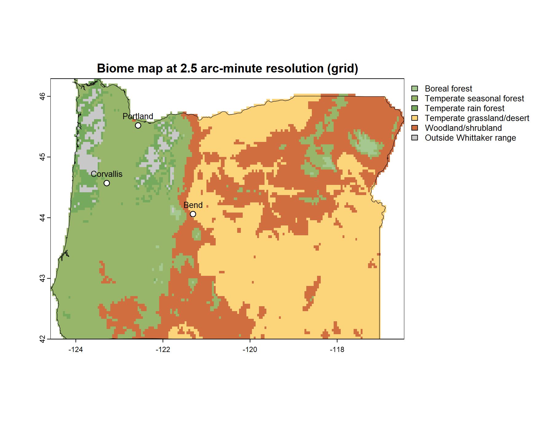
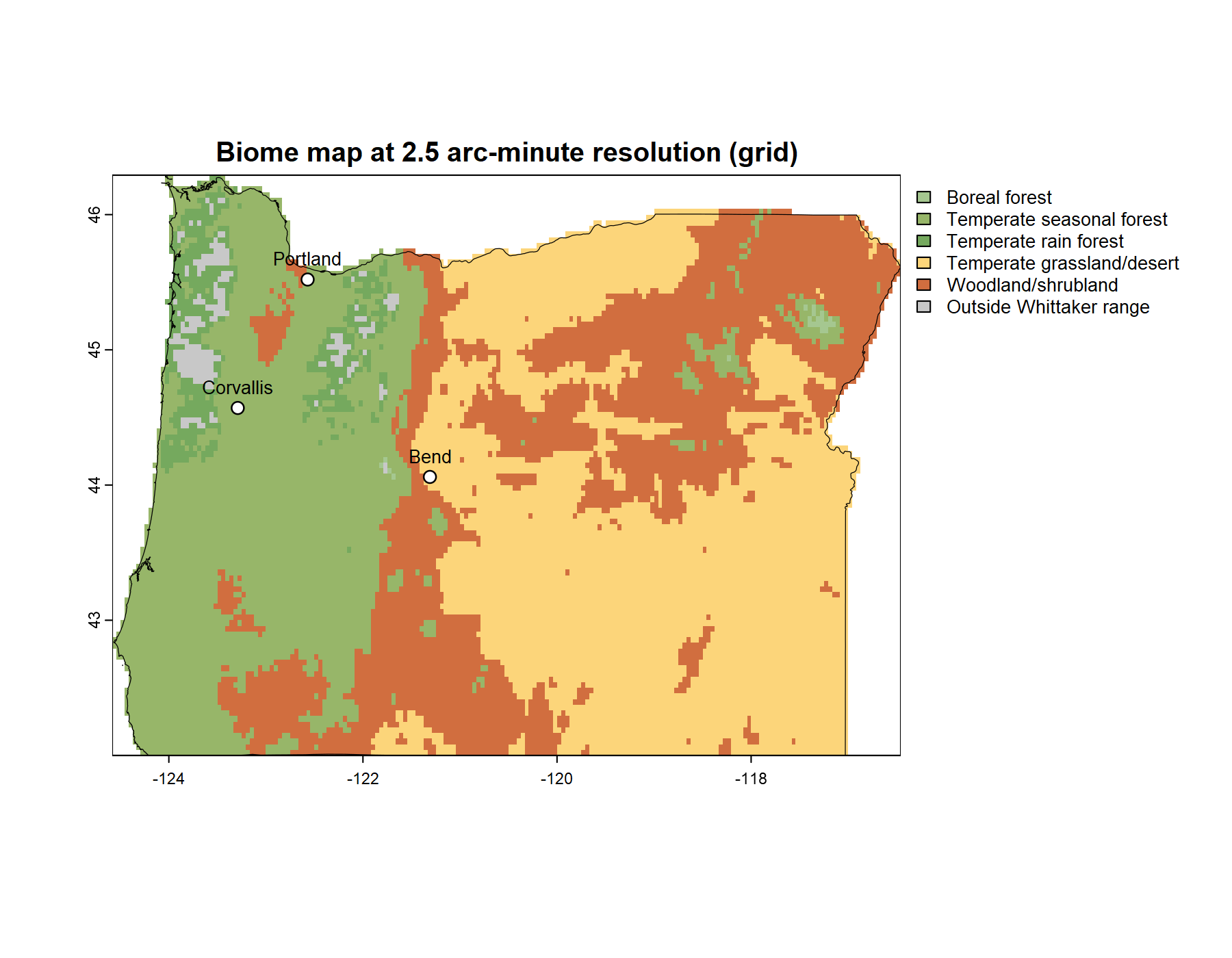
Compare the two maps city by city. A city well inside a biome shows the same color on both: its climate drifted, but not far enough to leave the region it began in. A city that sat near a boundary, in an ecotone, may show a different color on the second map. Its climate has crossed the line. Whether a place changes biome is a question of how close it stood to an edge, which is the spatial transition of the previous section and the temporal one of this section meeting in a single point.
The change is not confined to single points. The region’s whole composition re-weights. Run biome_composition() on the two maps and the dry biome, temperate grassland and desert, rises from about 36 to 39 percent of the state, while the forests give ground. The high cold pocket of boreal forest, already small at 0.7 percent under the historical climate, falls to almost nothing. The temporal transition is legible at the scale of one city and at the scale of the whole state at once.
One caution belongs with the figure. This is a single projection: one climate model, the middle-of-the-road SSP2-4.5 pathway, a mid-century window. It is a demonstration of what the tool can do at this scale, not a forecast. A higher-emissions pathway, or a later period, would move the maps further. The lasting value of the figure is the method it shows, mapping a classification forward in time, more than the particular numbers it produces.
A note on the marked points. These maps use cities, because a reader knows where Portland is, and a recognizable place makes a map easier to enter. An ecologist’s marked point would be something else. It would be the known location of a rare species, the site of a single vulnerable population. The question then stops being a demonstration. How close is that critical habitat to a transition zone? A population in the interior of its biome has room to absorb a shifting climate. A population whose climate already sits near a boundary has very little. The toolkit answers that question with the operations this chapter and the last have used, retrieve the biome, map the region, judge the distance to the edge. Only the stakes change.
The diagram and the map both draw biomes as regions with edges, and the edges are abstractions. They are also, in both senses this chapter has followed, the most alive part of the picture. In space, the ecotone is where diversity gathers. In time, the boundary is where a changing climate does its work, carrying places from one biome into another. A classification is most useful not when it is read as a set of boxes but when it is read as a field of gradients. The boundaries are where the gradient is steepest, and where the questions worth asking are.