4  Getting Started

This chapter installs the whittakerr package and confirms it runs. It is short by design. The work of the document is in the chapters that follow; this one makes sure the tools are in place before that work begins.

The whittakerr package is written in R. You will need a recent version of R, 4.0 or later, and any R working environment will do, though RStudio is the assumed setup. Basic familiarity with running R code is enough; the document explains the rest as it goes.

4.1 Installing whittakerr

The whittakerr package is not on CRAN. It is installed from GitHub, which requires the devtools package. If you do not already have devtools, install it first:

## devtools provides install_github(), used to install from GitHub
install.packages("devtools")

Then install whittakerr itself:

## load devtools, then install whittakerr from its GitHub repository
library(devtools)
install_github("kimbridges/whittakerr")

This is a one-time step. The install also pulls in the packages whittakerr depends on for climate-data access and spatial operations, including geodata, terra, and sf. Because of those dependencies, a first install can take several minutes.

A few of the document’s examples use packages that are not whittakerr dependencies, so they are not installed automatically. The main one is gt, which formats data tables for display; some chapters also use readr for reading data. Both are on CRAN:

## gt formats tables; readr reads data files; both are on CRAN
install.packages(c("gt", "readr"))

4.2 A first check

Once whittakerr is installed, load it at the start of any R session where you will use it:

## load whittakerr at the start of any session that uses it
library(whittakerr)

A quick check that the package is working. The name_biome() function classifies a single climate point (a temperature value and a precipitation value) into a Whittaker biome:

## classify a warm, moderately wet point into a Whittaker biome
name_biome(mean_temp_c = 25, total_ppt_cm = 250)

[1] "Tropical seasonal forest/savanna"

If that returns a biome name, the package is installed and running. One more check, this time a plot. The diagram is a ggplot2 plot, so load ggplot2 as well, then call plot_biomes() with no arguments to draw the Whittaker biome diagram itself:

## the diagram is a ggplot2 plot, so load ggplot2
library(ggplot2)
## draw the Whittaker biome diagram with no data points
plot_biomes()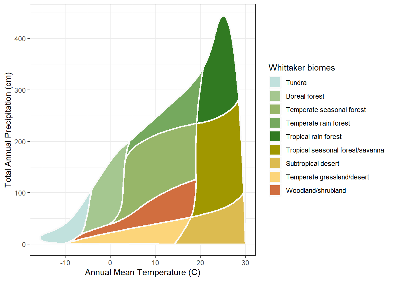

A colored diagram of the nine biomes in temperature-precipitation space means everything is in place. The rest of the document builds on these two functions and the others the package provides.

4.3 The setup chunk

Every chapter in this document that uses code begins with a setup chunk that loads the packages the chapter needs. The setup chunk is repeated at the start of each chapter so that any chapter can be opened and run on its own, without running the chapters before it. A typical setup chunk looks like this:

## the biome classification toolkit
library(whittakerr)
## WorldClim climate-data access
library(geodata)
## raster operations
library(terra)
## plotting
library(ggplot2)
## formatted tables
library(gt)

When you open a chapter and see a setup chunk, run it first. The rest of the chapter’s code depends on it. Not every chapter loads every package; the setup chunk for each chapter loads only what that chapter uses.

4.4 A note on units

One convention to know before going further: precipitation in whittakerr is always in centimeters. The Whittaker diagram’s vertical axis is annual precipitation, and the package follows the diagram’s native unit. When a function asks for total_ppt_cm, it wants centimeters.

Climate data from WorldClim arrives in millimeters. The get_climate() function, covered in the next chapter, returns precipitation in both millimeters and centimeters, so the conversion is handled for you. When you pass climate values into the biome functions, use the centimeter column.