Every ecological observation has a scale. So does every map, every diagram, every study design. Scale answers three questions about a piece of ecological work: how big is the area you looked at, how long did you watch it, and what level of organization were you describing. Three answers, every time, for every piece of work.
Scale is also rarely articulated. Researchers make scale choices reflexively, based on training and on what data they can get, and the choices are visible in the design but rarely defended in the prose. A typical paper presents its scale of analysis as if scale weren’t a decision at all. Modern landscape ecology and macroecology made scale central as a theoretical concept in the 1980s and 1990s, but the everyday habit of stating one’s scale and defending it hasn’t fully arrived.
The same observation looks different at different scales. Walking through a forest, an observer sees specific trees, particular birds, the patch of moss on a north-facing trunk. Standing back at a viewpoint, the same forest is a continuous green canopy meeting a ridge. From a satellite, it is one polygon in a national vegetation map, distinguished from the cropland next to it. All three observations are of the forest. Each answers a different question about it. The scales are not just zoom levels; they are different objects in the sense of being differently constituted for analysis.
This chapter argues that scale deserves explicit treatment, and shows what changes when it gets it. The previous chapter examined a biome as a category, what it does, why nine, why these axes, why life forms. This chapter asks one more question of the same diagram: at what scale does the biome category live? The answer involves three scales, not one, and Whittaker’s diagram makes specific choices on each. Once those choices are visible, the rest of the document becomes intelligible as a coherent scale-bounded enterprise rather than a series of arbitrary technical decisions.
3.1 The three scales
Three questions, three scales. Each is partly independent of the others.
The first is spatial: the size of the area in view. The vocabulary of spatial scale runs from microhabitat through habitat patch, landscape, region, continent, and finally global. A field site might be a 10-meter belt transect across a meadow, or a 5-kilometer grid cell at WorldClim resolution, or the whole Earth. The same vegetation can be studied at any of these scales, and the choice of which determines what variation is visible and what averages out.
The second is temporal: the duration of observation and the aggregation level of the resulting values. The vocabulary runs from instant through diurnal, seasonal, interannual, decadal, centennial, millennial, to geological. A weather observation is an instantaneous reading. An annual mean is a temporal aggregation that discards seasonal variation. A long-term normal, like the 1970–2000 average that WorldClim’s BIO1 uses, discards both seasonality and interannual variation. The temporal scale of the data shapes the temporal scale of the questions the data can answer.
The third is organizational: the level of biological structure being described. The vocabulary runs from individual through population, community, ecosystem, landscape, biome, and biosphere. An ecologist counting birds at a single site is doing population-level work. An ecologist measuring nitrogen flux through a forest is doing ecosystem-level work. An ecologist drawing biome polygons in temperature-precipitation space is doing biome-level work. Each level addresses different questions and uses different methods.
These three scales are partly independent. A study at landscape spatial scale can run at seasonal temporal scale and community organizational scale. Another study at the same spatial scale can run at decadal temporal scale and population organizational scale. Choices on the three axes are not bound to each other. This is part of what makes scale choices analyzable: they are three decisions, not one, and each can be examined and defended on its own.
3.2 The diagram’s three answers
The Whittaker diagram operates at three specific scales, one for each axis.
Spatially, it operates from regional to global. The climate values that go into the diagram are area averages, at WorldClim’s 2.5-minute resolution, roughly 5-kilometer grid cells. The polygons drawn on the diagram are built to be globally applicable: a temperature-precipitation pair from anywhere on Earth maps onto the same set of biome categories. Within-cell heterogeneity, such as the warmer pavement of a small city or the cold air pocket in a small valley, averages out of the data the diagram consumes.
Temporally, it operates at the long-term annual mean. BIO1 is mean annual temperature averaged over 1970–2000. BIO12 is total annual precipitation over the same period. Seasonality, interannual variability, individual drought years, and decadal climate oscillations are all discarded in this aggregation. The diagram answers questions about climate-vegetation relationships at the timescale where climate is treated as a stable property of place, not at the timescale of weather or even of single drought events.
Organizationally, it operates at the biome level. The categories are community-level vegetation types defined by life form. Species composition within a biome is not in view; ecosystem-level processes like nutrient cycling are not in view; individual organisms are not in view. The reader who wants to know about a particular species or a specific patch of forest is asking a question one or more organizational levels below where the diagram answers.
These choices are not defects. The diagram works precisely because the chosen scale is large enough to reveal patterns that exist across continents and small enough to keep a world map legible. The averaging is the scale choice. A diagram that retained every cell’s seasonality and every species’ identity would not be a diagram; it would be the raw data. Compression at this particular scale is what makes the relationship visible.
3.3 Oahu at two resolutions
A worked case from this document makes the point concrete. Oahu, the third-largest Hawaiian island, has dramatic climate variation across short distances. The windward Koolau Range receives over 7000 millimeters of annual precipitation. The leeward Waianae coast receives under 400 millimeters. The two coasts are about 50 kilometers apart.
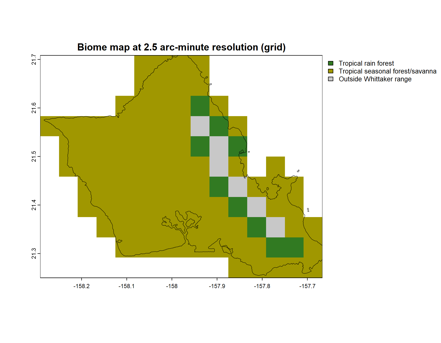
At 2.5-minute resolution, the standard the rest of this document uses, each climate cell averages conditions across a square roughly 5 kilometers on a side. The classification at this resolution is not uniform, but it is partial. Most of Oahu classifies as tropical seasonal forest/savanna. Along the windward Koolau crest, a band of cells classifies as tropical rain forest, and the wettest of those cells fall off the diagram entirely: their averaged precipitation is greater than anything in Whittaker’s envelope, and the classifier reports them, honestly, as outside its range. What the 2.5-minute map does not show, anywhere, is desert. Not one cell. The leeward dry pockets have vanished.
Oahu’s biomes at 2.5-arcminute resolution. Most of the island classifies as tropical seasonal forest/savanna; the windward Koolau crest shows as tropical rain forest and, in its wettest cells, as climate too wet for Whittaker’s diagram. No cell classifies as desert.
The pattern of what survives and what vanishes is not random. The windward wet crest survives because it is large: a whole mountain range’s worth of high precipitation, a feature tens of kilometers long. A 5-kilometer cell laid anywhere along it contains wet ground and little else, so it averages to wet. The leeward dry pockets vanish because they are small: a few square kilometers each, tucked against the coast. A 5-kilometer cell that catches a dry pocket also catches the wetter ground around it, and the wetter ground wins the average. Coarse resolution does not blur a landscape evenly. It keeps the large, strong features and discards the small ones. The grain of the data sets a size below which nothing can be seen.
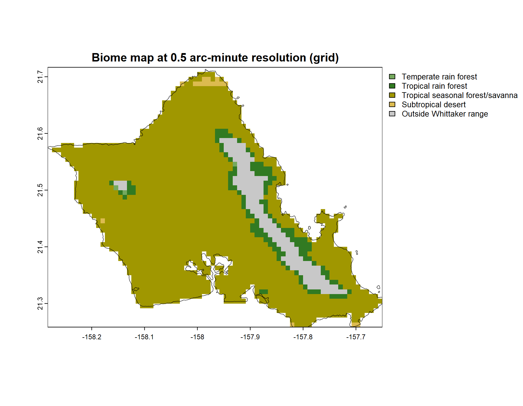
At 30-arcsecond resolution, about 1-kilometer cells, the grid is finally fine enough to fit inside a dry pocket. A cell can sit within one without reaching out to its wetter surroundings. The climate envelope at Kaena Point and along the lee of the Waianae Range falls inside Whittaker’s subtropical desert polygon, and the map shows desert assignments at exactly the locations local Hawaiian ecologists have long described as dry zones, the same zones that Mueller-Dombois wrote about in his vegetation studies of the islands.
Oahu’s biomes at 30-arcsecond resolution. The windward side is wet and the leeward side dry; and in the driest leeward pockets, too small to survive the coarser grid, the classifier now finds subtropical desert.
Same data, same classifier, same island. Two resolutions, two ecological pictures. At one scale Hawaii has deserts; at another it does not. The dry pockets are real either way. What changes is not the island but the grain, and the grain decides which truths about the island are visible and which average away.
This is the chapter’s prescription in a single worked case: name your scale, defend your scale, know what your scale obscures. The 2.5-minute analysis is not wrong. It is answering a different question than the 30-arcsecond analysis. A researcher characterizing the regional climate-vegetation relationship across the Pacific can use the coarser scale appropriately. A researcher hunting the dry refugia where xerophytic plants persist needs the finer one. The choice is part of the research, not prior to it.
3.4 Naming the rank
Taxonomists handle scale better than ecologists do, and they do it through an explicit hierarchy of ranks.
A taxonomist working with a plant identifies the rank at the start of the work: family, genus, species, with subspecies and varieties below. The choice of rank is methodological. A researcher who is studying genus-level patterns says so. A researcher who is studying species-level differences says so. The reader of a taxonomic paper knows immediately what unit of biological variation is in view because the rank is named.
The ranks themselves are stable. Linnaeus established the hierarchical structure in the eighteenth century, and the modern ranks (kingdom, phylum, class, order, family, genus, species) have been the standard vocabulary of biology for two centuries. New ranks have been added at the top (domain) and additional subdivisions below (subspecies, variety, form), but the structure has held. A reader of a taxonomic paper from 1850 and one from 2020 can talk to each other about rank.
Ecology has no equivalent. The vocabulary for spatial, temporal, and organizational scale exists, but it isn’t used with the same discipline. A paper that operates at the landscape scale rarely says so in those words. A paper that aggregates climate over decades rarely declares the temporal scale of its variables. A paper that works at the community level often presents its work as if “the system” were a single object rather than a choice of organizational level. The vocabulary exists; the discipline of using it doesn’t.
The chapter’s prescription is to borrow taxonomic discipline without taxonomic terms. Make scale explicit the way taxonomy makes rank explicit. The terms used should be ecology’s own (habitat patch, landscape, region, biome), not Linnaean ranks repurposed. But the practice should match: name the level, defend the choice, treat the level as a first-class methodological decision.
3.5 Words instead of ratios
Cartographers solve the scale-naming problem with ratios. Every printed map carries a scale notation: 1:10,000, 1:100,000, 1:1,000,000. The notation is rigorous. Two maps with the same ratio show the same amount of ground per centimeter of paper. A reader who knows the convention can compare maps confidently.
But cartographic ratios don’t carry intuitive content. Most readers can’t translate “1:1,000,000” into a felt sense of what they are looking at. The ratio is precise without being meaningful. For ecological writing, this is the wrong tradeoff. Ecologists work with material that is itself organized at named levels (habitat, community, ecosystem, biome), and these names already carry intuitive content. A reader knows roughly what a habitat is, what a community is, what a biome is. The terms do work that ratios don’t.
The pairing is straightforward. Approximate alignments are shown below.
Show the code
## gt renders the cartographic / ecological scale pairinglibrary(gt)## the rough alignment between cartographic ratios and the## named levels of ecological organizationscale_levels <-data.frame(cartographic =c("~1:10,000,000", "~1:1,000,000","~1:100,000", "~1:10,000","~1:1,000", "~1:100","~1:10"),ecological =c("Biome", "Region or ecoregion","Landscape", "Ecosystem","Community", "Population","Microhabitat"),visible =c("Climate-vegetation patterns; continental distributions","Multi-biome mosaics; large climate gradients","Habitat patches; mosaics; metacommunities","Community plus abiotic processes; energy and nutrient flow","Species composition; co-occurrence","Individual organisms; density","Within-individual conditions; sub-organism processes"))scale_levels |>gt() |>cols_label(cartographic ="Cartographic scale",ecological ="Ecological term",visible ="What is visible")
The ratios in the left column are illustrative, not strict. A landscape-scale study may be at 1:50,000 or 1:200,000 depending on the region’s size. The point is the rough alignment between cartographic scale and ecological term, not a one-to-one correspondence. A reader who knows ecological vocabulary can move down the table and feel the shift from continental to within-organism without needing to think in ratios.
The practical implication for ecological writing is simple. When stating the scale of work, use the ecological term. “Landscape-scale study,” “ecosystem-level analysis,” “community composition data.” The reader’s intuition about what each level contains gives the scale name immediate content. A cartographer would still need the ratios for printing a map at a precise size, and a quantitative ecologist might still need the ratios for spatial resolution calculations. But the cartographer’s reader thinks in ratios; the ecologist’s reader thinks in levels. The vocabulary should fit the audience.
3.6 A career across scales
David Goodall offers the cleanest case I have personally witnessed of scale awareness developing through practice.
Goodall (1914–2018) was an Australian-born plant ecologist, a pioneer of statistical methods in vegetation analysis, and productive into his second century. He was also my PhD advisor. After completing my degree, I served as Assistant Director under him in the US/IBP Desert Biome program, an NSF undertaking with a continental study scope. The advisor relationship came first; the program collaboration followed.
After running the Desert Biome program, Goodall moved his research focus to ecosystem-scale work. The migration was deliberate. He had spent years inside biome-scale science and knew, from inside, what biome-scale work delivered and what it averaged out. The dynamics within a single desert ecosystem (soil-moisture cycles, nutrient flows, the temporal pulses of productivity tied to rainfall events) were not visible in the broad climate-vegetation comparisons that justified biome-scale framing. Ecosystem-scale work could see them. The shift was an explicit scale choice made by a researcher who now knew the tradeoffs.
The migration is what scale awareness looks like over a career. A researcher who has worked at one scale has felt that scale’s limits in a way that no methodological essay can convey. The limits are not abstract; they are the specific questions the chosen scale couldn’t answer. Moving to a different scale is sometimes the right response to those felt limits. It isn’t abandonment of the earlier work. It is the same researcher, deliberately recalibrated, applying the same discipline at a different level.
A researcher needs to be aware of the scale at which they are working. Goodall’s career shows what that awareness can look like when the researcher takes it seriously across decades. This is the chapter’s prescription written across a career, not just a paper.
3.7 Making scale explicit
The chapter’s prescription is straightforward. State the scale of your work. Name the spatial extent and resolution. Name the temporal aggregation. Name the organizational level. Borrow the discipline of the taxonomist without the vocabulary, and use ecological terms that already carry intuitive content. Treat scale as a first-class methodological decision, not an inherited default.
What scale awareness gives you, beyond methodological hygiene, is access to a sequence of questions. The biome scale gives perspective: which categories exist, how they distribute across the planet, what the climate envelopes look like. The ecosystem scale gives mechanisms: how the nutrients cycle, how the productivity responds to rainfall, what processes underwrite the patterns visible from above. Once you have the perspective, it is natural to want the mechanisms. Goodall’s migration was the working out of exactly that progression.
For readers of this document, the scale choices are now visible. The Retrieving Climate Data chapter operates at 2.5-minute spatial resolution and 30-year temporal aggregation. The biome classification works at the community organizational level. The Build a Map and Beyond a Map chapters render at island and country spatial extents. The Draped on Topography chapter works at terrain-feature resolution within a country-scale extent. None of these is arbitrary. Each is a deliberate choice, defensible against the alternatives, and visible because this chapter named scale as something to name.
The rest of this document is one researcher’s set of scale choices. In the chapters that follow, scale is no longer the unstated dimension.