The Basic Whittaker Diagrams chapter showed how to read a site’s biome from the diagram: place the climate point, find the colored region that holds it. That is a visual act. It needs a person at the diagram, and it does not scale past the few points an eye can follow. This chapter does the same retrieval in code, where the biome comes back as a value a program can use.
Retrieval works at two scales. The narrow one is a single place: what biome is this point in? The wider one is a region: what biomes does this area hold, and in what proportion? The two are not separate questions. A point’s biome is a bare fact until it is read against its region. That a site is shrubland says little on its own; whether shrubland is most of the surrounding region or a rare pocket within it says a great deal. This chapter does both retrievals, the point and the region, and then closes on a question that neither answers.
8.1 Setup
Every code-bearing chapter begins with a setup chunk. Run it first.
Show the code
## the whittakerr toolkit: get_climate(), name_biome(), biome_composition()library(whittakerr)## ggplot2 for the composition bar chartlibrary(ggplot2)## read_csv() for the inline location tablelibrary(readr)## formatted tableslibrary(gt)## suppress read_csv() column-type messages for the whole chapteroptions(readr.show_col_types =FALSE)
8.2 The biome of one place
name_biome() is the retrieval function. It takes an annual mean temperature and an annual precipitation and returns the name of the biome whose region contains that climate. The climate itself comes from get_climate(), exactly as the climate chapter showed. Honolulu, the running example, in two steps:
Show the code
## retrieve Honolulu's climatehonolulu <-get_climate(lon =-157.86, lat =21.31)## retrieve the biome for that climatehonolulu_biome <-name_biome(mean_temp_c = honolulu$mat_c,total_ppt_cm = honolulu$map_cm)
name_biome() returns Tropical seasonal forest/savanna for Honolulu. This is the same answer that reading the diagram by eye would give, the region the point lands in, but now it is a value: a string a program can store, test, or hand to another function. The two arguments are mean_temp_c and total_ppt_cm, and get_climate() returns its values as mat_c and map_cm, so the climate columns feed straight in.
8.3 Several places at once
name_biome() classifies one point at a time. It rests on a point-in-polygon test, a single-point operation by nature. To retrieve biomes for a collection of places, apply it across them. The three Pacific-coast cities make the case.
Start with the cities as an inline table, one row per city:
Show the code
## three Pacific-coast cities, with their coordinatescities <-read_csv("name, lon, lat Honolulu, -157.86, 21.31 Los Angeles, -118.24, 34.05 Seattle, -122.33, 47.61")## show the tablegt(cities)
name
lon
lat
Honolulu
-157.86
21.31
Los Angeles
-118.24
34.05
Seattle
-122.33
47.61
The table holds a name and a pair of coordinates. get_climate() takes the coordinates and returns the climate:
Show the code
## retrieve the climate for all three cities in one callcities_climate <-get_climate(lon = cities$lon, lat = cities$lat)## show what get_climate() returnedgt(cities_climate)
lon
lat
mat_c
map_mm
map_cm
scenario
-157.86
21.31
24.70955
1253
125.3
historical
-118.24
34.05
18.82033
403
40.3
historical
-122.33
47.61
10.99050
1012
101.2
historical
get_climate() is vectorized, so the one call retrieved all three climates. The two columns to carry forward are mat_c, the annual mean temperature, and map_cm, the annual precipitation in centimeters. Apply name_biome() to each city:
Show the code
## name_biome() takes one point; mapply() applies it to each## city's temperature (mat_c) and precipitation (map_cm)cities$biome <-mapply(name_biome,mean_temp_c = cities_climate$mat_c,total_ppt_cm = cities_climate$map_cm)## collect each city with its retrieved biomecity_biomes <-data.frame(City = cities$name,Biome = cities$biome)## show the tablegt(city_biomes)
City
Biome
Honolulu
Tropical seasonal forest/savanna
Los Angeles
Subtropical desert
Seattle
Temperate seasonal forest
name_biome() is not vectorized, so mapply() carries it across the rows, pairing each city’s mat_c with its map_cm. The biome is attached to cities as a new column, and the small table pairs each city with its result. Three cities, three biomes.
8.4 A point in its region
A retrieved biome is a fact about a point. It gains meaning when it is set against the region the point sits in. Take Bend, in central Oregon:
Show the code
## retrieve the climate and biome for Bend, Oregonbend <-get_climate(lon =-121.31, lat =44.06)bend_biome <-name_biome(mean_temp_c = bend$mat_c,total_ppt_cm = bend$map_cm)
name_biome() returns Temperate grassland/desert for Bend. That is the point retrieval, the same operation as before, and it leaves a question open. Is Temperate grassland/desert what most of Oregon is, so that Bend sits in ordinary country, or is it a minority biome, so that Bend is an unusual spot in a region mostly of something else? The point retrieval cannot say. A regional retrieval can.
biome_composition() answers it. It needs a biome map of the region. Building one is the Mapping chapter’s subject; for this chapter it is enough to build the Oregon map once, and to reuse it if it has already been built:
Show the code
## Build the Oregon biome map, but only if it is not already## in memory. exists() tests for the variable; if an earlier## run left oregon_map in place it is reused, otherwise it is## generated here. map_biomes() is covered in the Mapping## chapter.if (!exists("oregon_map")) { us_states <- geodata::gadm(country ="USA", level =1,path ="cache/gadm_cache") oregon <- us_states[us_states$NAME_1 =="Oregon", ] oregon_map <-map_biomes(oregon, resolution =2.5)}
The exists() test is what lets the chapter stand on its own. Run it fresh and it builds the map; run it again, or after another chapter has already built oregon_map, and it reuses what is there. The costly step happens once.
With the map in hand, biome_composition() retrieves the breakdown:
Show the code
## retrieve the biome composition of the Oregon maporegon_composition <-biome_composition(oregon_map)## show what biome_composition() returnedgt(oregon_composition)
biome
n_cells
area_km2
percent
Temperate grassland/desert
5886
91584.5
35.9
Temperate seasonal forest
4869
75393.9
29.5
Woodland/shrubland
4598
71007.8
27.8
Temperate rain forest
630
9584.1
3.8
Outside Whittaker range
400
6066.4
2.4
Boreal forest
112
1712.6
0.7
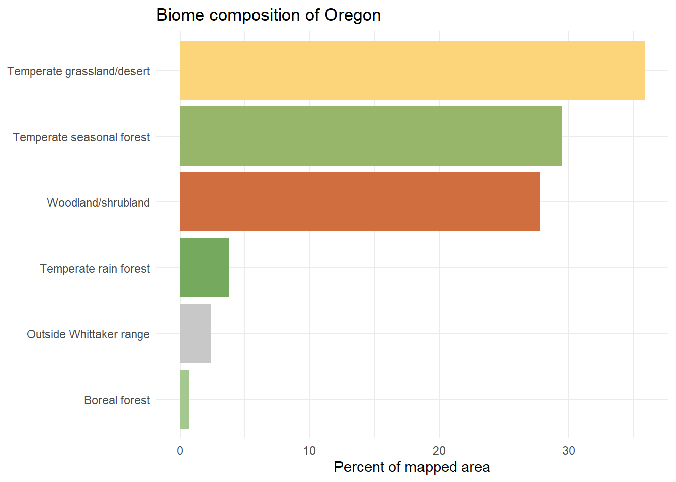
One row per biome, with the cell count, the area in square kilometers, and the percentage share of the mapped region. The shares read more readily as a chart:
Show the code
## one color per biome, with the fixed gray for unclassified landbar_colors <-setNames(biome_palettes$ricklefs, biome_palettes$biome)bar_colors["Outside Whittaker range"] <-"#C8C8C8"## a horizontal bar chart, bars ordered by shareggplot(oregon_composition,aes(x = percent, y =reorder(biome, percent), fill = biome)) +geom_col() +scale_fill_manual(values = bar_colors, guide ="none") +labs(x ="Percent of mapped area", y =NULL,title ="Biome composition of Oregon") +theme_minimal()
Now Bend’s biome can be read in context. Find Temperate grassland/desert among the bars. A long bar means Bend sits in the biome that defines most of the region, an ordinary location for that part of Oregon. A short bar means the opposite: Bend is a pocket, a site whose biome is the exception around it. The point retrieval found the biome; the regional retrieval found whether the biome is typical. This pairing of the point and the region is a major use of the toolkit. In place-oriented work the composition gives a point its context; in region-oriented work, in the Mapping chapter, the same function describes a region in its own right.
8.5 What the name leaves out
name_biome() answers one question well and is silent on a second. It performs a point-in-polygon test: it finds the biome region that contains the climate point and returns that biome’s name. A point a hair inside a boundary and a point deep in a biome’s interior receive the identical answer. The name does not tell them apart.
Yet they are not in the same situation. The interior point sits in climate that is firmly its biome’s. The boundary point sits in climate that is nearly a neighbor’s, and a modest shift, the kind a changing climate produces, would carry it across the line. For a botanical garden, that is the difference between planting assumptions that are secure and ones that are precarious. Retrieval returns the category; it does not return the distance to the category’s edge.
That distance is where the next questions live. A biome does not stop at a line so much as give way across a zone, and the sites within that zone, the ecotones and the climate-marginal places, are where the most is at stake. Retrieval names the biome, and the name is a beginning rather than an end. The chapters that follow ask what the name contains and how firmly it holds.