Show the code
## the whittakerr toolkit: map_biomes(), smooth_biome_map(),
## export_biome_kml()
library(whittakerr)Years ago I drove from Nairobi to the Maasai Mara. The road ran rutted through the highlands, and then it dropped — one long fall to the floor of the Great Rift Valley. It was an experience in both space and time — a descent through the country, and a descent into deep time, because the Rift is where humankind likely began. It is hard not to be awed, landing on that ground.
And then, in the middle of the valley, two huge satellite dishes — the Longonot Earth Satellite Station, a degree or so south of the equator. They were a ground station for talking with satellites: technology set down in the cradle of our species, and a geographic reminder of the shape of our planet. They are quiet now — fiber-optic cable took over the work the dishes once did. Along the same road, zebras, giraffes, a host of other animals. A clash of old and new. A spellbinding sight.
Underneath the awe, that drive was a lesson in topography — not topography read off a map, but topography moved through, felt in the long descent and measured by the hour it took. Every biome map this document has built has been flat. A flat map is a true and useful thing, but it is not the Earth. The Earth has the shape the Rift Valley has: relief, slope, a third dimension that climate answers to.
This chapter puts the flat map back on that shape. It takes the Kenya biome map of the previous chapter — the one anchored, measured, and smoothed there — and drapes it over the real, three-dimensional Earth, using a tool of the same family as those dishes in the valley: satellite technology that holds the actual shape of the planet. What the draping reveals is the chapter’s subject, and it is more than a better-looking picture.
## the whittakerr toolkit: map_biomes(), smooth_biome_map(),
## export_biome_kml()
library(whittakerr)This chapter works from the Kenya biome map of the previous chapter. It is rebuilt here, if an earlier run has not left it in memory, so the chapter can be opened on its own. The recipe is the one Build a Map walked through.
## rebuild the Kenya biome map if it is not already in memory
if (!exists("kenya_map")) {
  ## a whole country is one GADM polygon: level 0, no crop
  kenya     <- geodata::gadm(country = "KEN", level = 0,
                             path = "cache/gadm_cache")

  ## classify every cell at 2.5-arcminute resolution
  kenya_map <- map_biomes(region_polygon = kenya,
                          resolution     = 2.5)
}It is worth being exact about what the Kenya biome map was built from, because the chapter’s test rests on it. The classifier read two numbers for each cell of the country — the annual mean temperature and the annual precipitation — and nothing else. The Whittaker biomes are regions of a temperature-precipitation space; name_biome() does one thing, which is to find the region a cell’s two numbers fall in. Elevation is not an input. Slope, aspect, the line of a ridge, the bulk of Mount Kenya: none of it is anywhere in the machinery. The map of Kenya’s biomes was drawn without the mountains.
That blindness is not a flaw to apologize for. It is what gives the coming test its force. A classifier handed elevation would trace the mountains trivially — a map that already knows where the peaks are will of course follow them, and prove nothing by it. This classifier was handed no such thing, only two bare numbers per cell. So if its map turns out to fit the terrain, the fit cannot have been arranged.
A fit is possible at all because climate is not independent of terrain. It is, to a striking degree, made by it. Air cools as it rises — very roughly six degrees for every thousand metres — so a mountain is cold at the top. Mount Kenya climbs past five thousand metres; by that rate its summit stands some thirty degrees colder than the coast at Mombasa, cold enough, almost on the equator, for ice. And rain is wrung from air forced upward, so a slope facing the wind runs wet while the country in its lee runs dry. Orography writes itself into temperature and into precipitation — the two numbers the classifier read.
So there is a chain, and the classifier sits in the middle of it blind. Terrain shapes climate; climate is what the classifier reads; the classifier returns the biome map. It cannot see the first link, and it does not need to, because by the time the climate reaches it the first link has already done its work. The biome map, built without the mountains, carries the mountains anyway — secondhand, smuggled in through the climate.
That is what makes a test possible. Lay the map back on the real, three-dimensional terrain. If the biomes have come to rest where the terrain would put them — the cold biomes high on the massifs, the dry biomes in the rain shadows, the boundaries tracking the ridgelines — then the classifier read the climate correctly. It must have: a misread climate could not recapitulate a mountain the classifier never knew was there. The terrain is a witness the classifier never consulted, and draping the map is how we put it on the stand.
This is a different verification from the one the previous chapter used. Beyond a Map checked the map at its anchors — Nairobi, Mombasa, the Mara — against what a person knows of those places, and such a check reaches exactly as far as that knowledge reaches. The topographic test calls a different witness: the land itself. The physics that ties climate to terrain holds in every cell of the map, so the land can testify everywhere at once — over the empty country no one in particular can speak for as much as over the famous parks. It is a real test, too, not a flattering one. It can fail, and where it fails there is something to learn. That is the chapter’s second half.
Putting the witness on the stand takes one function. export_biome_kml() turns a biome_map into a KML file — the format Google Earth reads — with the biomes written as colored polygons.
The export works best from a smoothed map. The previous chapter showed that smoothing the Kenya country map is the benign case: the biome regions are broad, and the smoothed boundaries read as boundaries rather than as the staircase of a grid. On three-dimensional terrain that matters more, not less — a stepped grid edge draped over a hillside looks like a rendering fault. So the map is smoothed first, then exported.
## smooth the Kenya map; smoothed boundaries drape over
## terrain more naturally than the stepped grid edges
kenya_map <- smooth_biome_map(kenya_map)

## write the biome map as a KML file for Google Earth
export_biome_kml(kenya_map,
                 file = "kenya_biomes.kml",
                 name = "Kenya Biome Map")
Two details of that file are worth knowing, because they are what make this a drape and not a flat sheet laid over the country. Each polygon is written to clamp to the ground and to tessellate — instructions that tell Google Earth to set the polygon on the terrain surface and let it follow every rise and fall of that surface, instead of holding it flat. And the fill is semi-transparent, so the land shows through the color. The result is the biome map lying on Kenya the way a cloth lies on what it covers.
To see it, open kenya_biomes.kml in Google Earth. The biome map appears on the globe; tilt the view from straight down toward the horizon, and the flat map becomes a landscape — the highlands rising, the Rift trenched into the country, the biomes riding the terrain beneath them.
That tilt is the chapter’s whole subject, and a screenshot only half carries it. So the file is yours to take: download kenya_biomes.kml, open it in Google Earth, and turn the country in your own hands. The next section reads what the turning shows — but the reading goes better with the globe in front of you.
Earlier, this chapter framed a test and left it hanging: would the biomes, draped on the real terrain, come to rest where the terrain would put them? The KML is open in Google Earth now, and the answer can be read off the tilted globe. At the broad scale it is plainly yes — the cool, wet highlands carry the forest biomes, the hot lowlands carry the dry ones, and the country sorts itself the way its relief says it should. But the broad scale is the easy case. Two places repay a closer look.
The first is Mount Kenya.
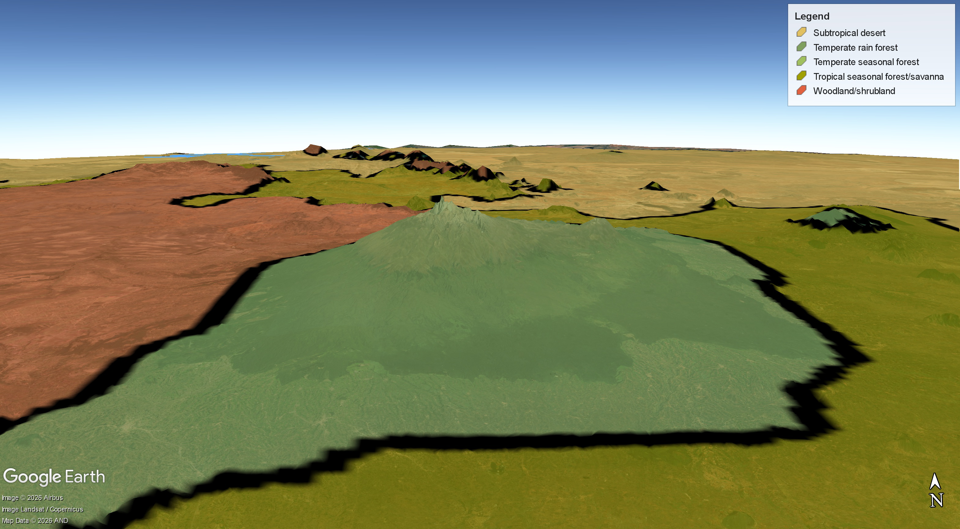
Consider what the classifier did here. It never knew Mount Kenya existed; it read two numbers for each cell and matched them to a Whittaker polygon. Yet the forest biome it assigned, draped on the terrain, is the mountain: the green polygon’s edge runs around the massif’s foot, and everything within that edge is the mountain itself. The polygon and the landform are one object. The classifier did not draw a mountain because it was told to. It drew a mountain because a mountain is cool and wet, cool and wet is what its two numbers reported, and the Whittaker scheme answers cool and wet with forest. The terrain stood upstream of the climate, the climate upstream of the biome, and so the biome came out mountain-shaped.
The polygon’s edge makes the same point a second way. Where it crosses Mount Kenya’s steep lower slopes it thickens into a dark band — the edge, clamped to the ground, climbing through a great deal of elevation in a short horizontal distance. On the flat country it is a thin line; on the mountain’s flank it is a wide dark stripe. The width of the edge is a reading of the steepness it crosses. The rendering is not only showing the verification; in that dark band it is displaying the very mechanism, orography, that the verification rests on.
The second place is the Great Rift Valley.
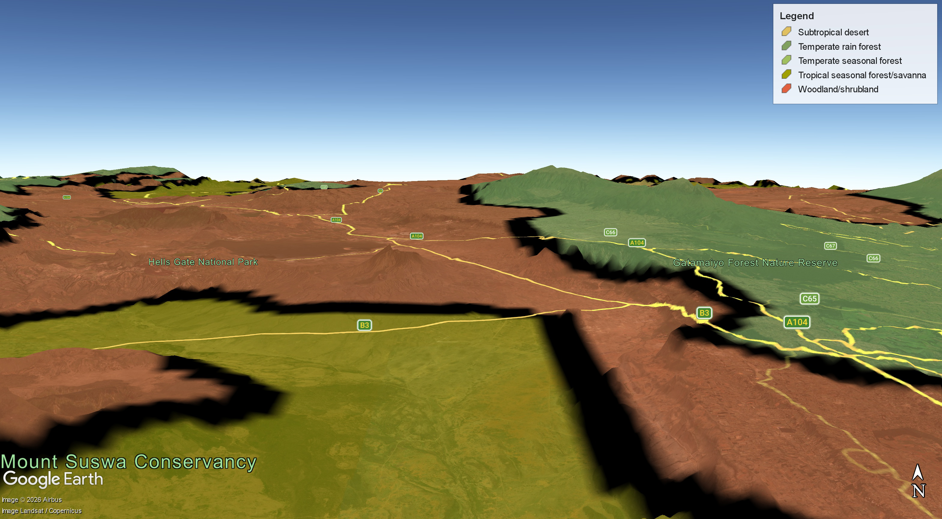
This is the country of the chapter’s opening, the long drive down into the Rift, and the drape shows what that drive moved through. The high rim, where the air is cool and the rain is caught, holds the forest biome. Below it the country dries: down the escarpment and across the valley floor the map turns to woodland and shrubland, and to tropical savanna. The boundary between the high forest and the dry valley runs along the lip of the escarpment — the line on the map and the break in the land are the same line.
The B3 highway threads down off the rim and out across the valley floor — the road this chapter opened on. To follow it on the drape is to retrace the opening’s descent: every biome boundary the road crosses is a climate boundary the drive passed through, felt at the time as nothing more than the air warming and the country drying. The escarpment throws the dark edge-bands again, broad where the wall is steep. The Rift — the deepest topographic fact in this part of Africa — has been written into the biome map by a classifier that knew only the weather.
So the answer is yes. The map fits the terrain, and fits it well enough that the terrain can be read back out of it. A classifier given two numbers for each cell, and nothing whatever about the shape of the land, has drawn Mount Kenya and traced the Rift. The verification the chapter set up has been met. That is the fit — and it is not the whole of what the drape shows. The next section turns to the rest.
So far, the draping has shown agreement: the biome map fit the terrain, and the fit verified the classifier. But the chapter set out to run a real test, and a real test is one that can come up short. So the honest question now is where the map and the Earth do not line up. They fail to line up in two different ways. Neither is a flaw to be hidden; both are the map still doing useful work.
The first is the line that was expected and is not there. Pick out a modest mountain on the terrain, or a low ridge, and look to the draped map for a biome boundary along its crest. Sometimes there is none: the map runs straight through, the same biome on both sides. The topography was real, but it was not enough — it did not lift the air far enough to cool it past a Whittaker boundary, or the rain it might have wrung from the sky had already been spent on some range upwind. The classifier missed nothing; the gradient simply was not there to be drawn. We get what the Earth’s complex processes deliver, and sometimes what they deliver is no line at all.
Carried to its limit, that becomes the test’s own guarantee. Over genuinely flat country — a plain with no orography to speak of — the draped map shows no topographic signal whatever, because there is none to show. A test that can come up empty is a test that was not arranged to pass. The clean fits of Section 5 carry their weight precisely because this emptiness was always possible.
The second kind of disagreement is quieter, and more interesting. Here the climate gradient is real, the classifier read it correctly, and the biome the map assigns is the right answer for the climate — and yet the living ecosystem on the ground is not quite what the biome name implies. The Maasai Mara is the case to hold in mind. The map gives the Mara a savanna biome, and savanna is indeed what is there. But the Mara’s open grassland, its plains kept clear for the great herds, is not the work of climate alone. Fire holds it open — fire from lightning, and fire set by people for many centuries — and so do the animals themselves, the grazers and the elephants that push the young trees down. Left to its climate, with neither fire nor herds, the Mara would carry more wood than it does. The biome label is true. It is also incomplete.
That incompleteness is not a defect to be corrected; it is the most useful thing a simple classifier does. Because the map reads only temperature and precipitation, every place where the ground departs from the climate’s prediction is a place where some other force is at work — and the departure points straight at it. Fire here; a serpentine soil there; a ribbon of gallery forest along a river the climate raster was too coarse to catch. A classifier that somehow folded all of those forces in would have no mismatches left, and so would point nowhere. This one, by staying simple, keeps a set of signposts. The biome map is the coarse cut; its mismatches mark where the finer work begins — the study of the ecosystem itself, the level beneath the biome.
So the draped map does more than confirm. Where it agrees with the terrain, it verifies the climate reading, as it did at Mount Kenya and the Rift. Where it disagrees, it is informative still: it reports either that the Earth delivered no gradient to draw, or that something beneath the climate is shaping the land. Agreement confirms; disagreement instructs; both are the map doing its work.
This chapter set out to test the biome map against the planet, and the test is done. The Kenya map was draped on Google Earth and read against the terrain. At Mount Kenya the forest biome and the mountain were the same shape; across the Rift the biomes stacked by the relief, their boundaries running with the escarpment. Where the map agreed with the land it verified the classifier; where it disagreed it pointed past itself — to a gradient the Earth never delivered, or a fire the climate could not see. The question the previous chapter handed forward — whether a classification that never saw a mountain had nonetheless drawn one — has its answer. It had.
There is a longer arc closing here as well. The Build a Map chapter looked back to a darkroom of rubylith and copy cameras, where a single thematic map was a week of skilled handwork, and to the moment computing lifted that cost away. Computing was one transformation. This chapter has arrived at the next. The biome map here was not cut by hand, and not merely computed and printed flat; it was laid on the turning globe and tilted into a landscape. Cut, computed, draped — three ways to make a map, and a single working life has reached across all of them.
The document’s own journey closes with it. It began at the Whittaker diagram, where climate is lifted off the Earth into a space of two axes and a biome becomes a region of temperature and precipitation. It moved to the biome map, the classification laid back down on geography, though still flat. It ends here, with that map set on the real, three-dimensional planet the climate was drawn from in the first place. A diagram, a map, a map on the Earth: the classification has gone all the way out into abstraction and all the way home to the ground.
One chapter remains. The map has been built, read, and now tested, and it holds. What is left is to step back — to remember that the lines drawn so convincingly across Mount Kenya and the Rift are lines we drew, and to look again at the country that lies, always, in between them.