Think about where you buy groceries. If the markets are all about the same, you go to the nearest one. Draw a line around everyone who shops at each market and you’ve divided the town into districts. Every household inside a district is closer to its own market than to any other.
That’s a Voronoi tessellation. Each point, here a market, gets a tile. The tile holds every place that’s closer to its point than to any other point. The tiles fit together with no gaps and no overlaps, and together they cover the whole area.
This chapter builds one twice. First with five imaginary markets, small enough to see how it works. Then with twelve vegetation samples at Kīpuka Puaulu, which gives the map that opened Chapter 1.
Show the code
## --- Standard packages ---## many useful functions, including read_csv() and ggplot()library(tidyverse)## formatted tableslibrary(gt)## --- Specialized packages ---## spatial data: points, polygons, and the Voronoi functionlibrary(sf)## --- Options and defaults ---## suppress read_csv() column-type messagesoptions(readr.show_col_types =FALSE)## the vegetation colors used throughout the document (Okabe-Ito palette)veg_colors <-c("Kīpuka forest"="#009E73","Koa-ʻōhiʻa forest"="#0072B2","ʻŌhiʻa forest"="#56B4E9","ʻŌhiʻa scrub"="#E69F00","Grass and savanna"="#F0E442")
2.1 Five markets
Here are five markets in a square town, ten kilometers on a side. The coordinates are in kilometers from the town’s southwest corner.
Show the code
## five markets, their positions in kilometersmarkets <-read_csv(file ="market, easting, northing A, 2.0, 8.0 B, 7.0, 8.5 C, 5.0, 5.0 D, 1.5, 2.0 E, 8.0, 2.5")## show the data as a tablemarkets |>gt() |>tab_source_note(source_note ="Imaginary markets, for demonstration.")
market
easting
northing
A
2.0
8.0
B
7.0
8.5
C
5.0
5.0
D
1.5
2.0
E
8.0
2.5
Imaginary markets, for demonstration.
Three steps turn the points into tiles. The first builds the tiles. The second splits the result into one polygon per market. The third trims the tiles to the edge of town, because a tile on the outside of the group would otherwise run on forever.
Show the code
## turn the table into spatial pointsmarket_points <-st_as_sf(markets, coords =c("easting", "northing"))## the town: a square, 10 km on a sidetown_box <-st_bbox(c(xmin =0, ymin =0, xmax =10, ymax =10))town <-st_as_sfc(town_box)## step 1: build the tiles around all the points at oncetiles_all <-st_voronoi(st_union(market_points), envelope = town)## step 2: split the result into separate polygonsmarket_tiles <-st_collection_extract(tiles_all)## step 3: trim the tiles to the town's edgemarket_tiles <-st_intersection(market_tiles, town)## the tiles come back in their own order, so attach each tile to the market inside itmarket_tiles <-st_sf(geometry = market_tiles)market_tiles <-st_join(market_tiles, market_points)## draw the tiles, the markets, and their labelsggplot() +geom_sf(data = market_tiles, fill ="grey92", color ="grey30") +geom_sf(data = market_points, size =2.5) +geom_sf_text(data = market_points, aes(label = market), nudge_y =0.45, size =4.5) +coord_sf(expand =FALSE) +theme_minimal(base_size =13) +labs(x =NULL, y =NULL)
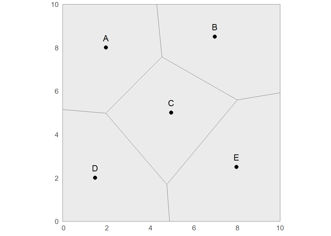
Five markets and their tiles. Every place inside a tile is closer to that tile’s market than to any other.
2.2 Halfway
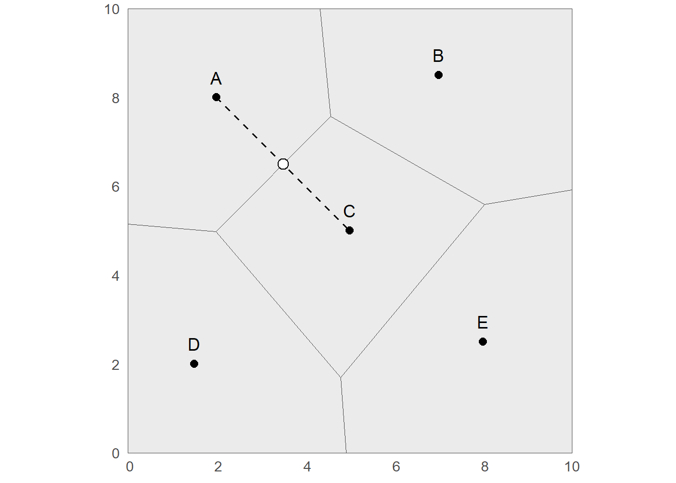
Look at the edge between markets A and C. Every place on it is exactly as far from A as from C. That makes it the line that cuts the path between them in half, at a right angle. Each edge in the map is built the same way, from one pair of neighboring points.
The midpoint between A and C is easy to find: average their coordinates.
Show the code
## the two marketspair <-filter(markets, market %in%c("A", "C"))## the midpoint of the path between themmidpoint <-tibble(easting =mean(pair$easting),northing =mean(pair$northing))## show the midpoint as a labelled tablemidpoint |>gt() |>tab_header(title ="Midpoint between markets A and C (km)")
Midpoint between markets A and C (km)
easting
northing
3.5
6.5
The edge between A and C crosses the path between them (dashed) at its midpoint (open circle), at a right angle.
Show the code
## the path from A to C, as a one-row table of start and end pointspath <-tibble(x = pair$easting[1], y = pair$northing[1],xend = pair$easting[2], yend = pair$northing[2])## draw the tiles again, with the path from A to C and its midpointggplot() +geom_sf(data = market_tiles, fill ="grey92", color ="grey30") +geom_segment(data = path, aes(x = x, y = y, xend = xend, yend = yend),linetype ="dashed") +geom_point(data = midpoint, aes(easting, northing), shape =21, fill ="white", size =3.5) +geom_sf(data = market_points, size =2.5) +geom_sf_text(data = market_points, aes(label = market), nudge_y =0.45, size =4.5) +coord_sf(expand =FALSE) +theme_minimal(base_size =13) +labs(x =NULL, y =NULL)
The edge between A and C crosses the path between them (dashed) at its midpoint (open circle), at a right angle.
So a Voronoi map makes one assumption about the ground between the points. Whatever is true at a point is true halfway to its neighbors. Past the halfway line, the neighbor takes over.
2.3 What the map uses, and what it doesn’t
A Voronoi map uses three things and nothing else:
where the points are,
what category each point belongs to, and
the border of the study area.
It doesn’t know about roads, rivers, ridges or lava flows. If a river runs between two markets, the tile edge crosses it anyway. For markets, that might be a real weakness. People don’t shop across a river with no bridge.
The method has several names, because it was found more than once. Mathematicians know it from the work of Peter Gustav Lejeune Dirichlet in 1850 (Dirichlet 1850) and Georgy Voronoi in 1908 (Voronoi 1908). Geographers and hydrologists often say Thiessen polygons, after Alfred Thiessen, who used them in 1911 to average rainfall from a scatter of rain gauges (Thiessen 1911). It’s the same construction under each name.
It’s fair to call the result reproducible. It’s not quite fair to call it objective. Someone chose where the points went and where the border runs, and those choices shape every tile. But anyone given the same points and the same border gets exactly the same map. That’s what a hand-drawn map can’t promise.
2.4 Twelve points at Kīpuka Puaulu
Now the same steps with real ground. The twelve sample points below are spread across a 3.2 by 2.6 kilometer rectangle around Kīpuka Puaulu. I placed them for this demonstration, three in each of four kinds of vegetation structure, and each one takes the vegetation type that the 1974 map shows at that spot. Later chapters replace them with real relevés.
The coordinates are in meters, in the UTM zone 5 north system that covers the island of Hawaiʻi.
Show the code
## the twelve sample pointsreleves <-read_csv("data/kipuka_puaulu_releves.csv")## show themreleves |>gt() |>tab_source_note(source_note ="Points placed for demonstration; vegetation types from Mueller-Dombois and Fosberg (1974).")
releve
easting
northing
vegetation
R01
257004.4
2152223
Koa-ʻōhiʻa forest
R02
257424.4
2151038
ʻŌhiʻa scrub
R03
257534.4
2150198
ʻŌhiʻa scrub
R04
259494.4
2151803
ʻŌhiʻa forest
R05
258879.4
2151398
ʻŌhiʻa forest
R06
257084.4
2150703
ʻŌhiʻa scrub
R07
256834.4
2151818
ʻŌhiʻa scrub
R08
258819.4
2151733
Grass and savanna
R09
258414.4
2151578
Kīpuka forest
R10
257284.4
2152133
Koa-ʻōhiʻa forest
R11
258074.4
2151483
Kīpuka forest
R12
258049.4
2151043
Grass and savanna
Points placed for demonstration; vegetation types from Mueller-Dombois and Fosberg (1974).
Show the code
## the study area, given by its southwest and northeast cornersarea_corners <-read_csv("data/kipuka_puaulu_study_area.csv")## show itarea_corners |>gt() |>tab_header(title ="Study area corners (UTM zone 5N, meters)")
Study area corners (UTM zone 5N, meters)
corner
easting
northing
southwest
256666.9
2149895
northeast
259866.9
2152495
The steps are the ones used for the markets. The only change is that the points now carry a coordinate system, EPSG code 32605, so distances come out in meters.
Show the code
## turn the table into spatial points in UTM zone 5Nreleve_points <-st_as_sf(releves, coords =c("easting", "northing"), crs =32605)## the study area as a rectanglestudy_box <-st_bbox(c(xmin = area_corners$easting[1],ymin = area_corners$northing[1],xmax = area_corners$easting[2],ymax = area_corners$northing[2]),crs =st_crs(32605))study_area <-st_as_sfc(study_box)## step 1: build the tilestiles_all <-st_voronoi(st_union(releve_points), envelope = study_area)## step 2: split into separate polygonsreleve_tiles <-st_collection_extract(tiles_all)## step 3: trim to the study areareleve_tiles <-st_intersection(releve_tiles, study_area)## attach each tile to the point inside itreleve_tiles <-st_sf(geometry = releve_tiles)releve_tiles <-st_join(releve_tiles, releve_points)## draw the mapggplot() +geom_sf(data = releve_tiles, aes(fill = vegetation), color ="white", linewidth =0.6) +geom_sf(data = releve_points, shape =21, fill ="white", color ="black", size =2.4) +geom_sf_label(data = releve_points, aes(label = releve), nudge_y =110, size =3,label.padding =unit(0.1, "lines"), fill ="white") +scale_fill_manual(values = veg_colors, breaks =names(veg_colors), name =NULL) +coord_sf(datum =NA, expand =FALSE) +theme_void(base_size =13) +theme(legend.position ="bottom")
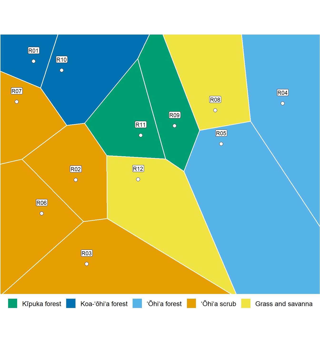
The twelve points and their tiles, colored by vegetation type. This is the map that opens Chapter 1.
A map made of tiles also gives numbers. Each tile has an area, so each vegetation type does too.
Show the code
## the area of each tile, converted from square meters to hectaresreleve_tiles <-mutate(releve_tiles, area_ha =as.numeric(st_area(geometry)) /10000)## drop the geometry and add up the area by vegetation typearea_by_type <-st_drop_geometry(releve_tiles)area_by_type <-group_by(area_by_type, vegetation)area_by_type <-summarise(area_by_type, tiles =n(), area_ha =round(sum(area_ha), 1))area_by_type <-arrange(area_by_type, desc(area_ha))## show the resultarea_by_type |>gt() |>tab_header(title ="Area by vegetation type, from the tiles")
Area by vegetation type, from the tiles
vegetation
tiles
area_ha
ʻŌhiʻa forest
2
260.5
ʻŌhiʻa scrub
4
248.3
Grass and savanna
2
149.3
Kīpuka forest
2
88.8
Koa-ʻōhiʻa forest
2
85.1
Those numbers are only as good as the assumption behind them. Twelve points can’t know what lies between them. The halfway rule fills that ground in, whether the vegetation agrees or not.
2.5 Where the assumption fits
For markets and schools, the halfway rule is close to how people behave. You shop at the nearest market and your children go to the nearest school, most of the time.
For soils, Arnold and Milne (1984) found that it matched what the cartographer already did. With a sample every 50 to 200 meters, a hand-drawn soil map is close to a Voronoi map anyway.
Vegetation is harder. Relevés are expensive, so they’re far apart. And the vegetation scientist drawing the map doesn’t draw halfway lines. The line goes where the edge of the forest shows on the air photo. That’s the gap between the two maps in Chapter 1, and it’s why the question there is a real one.
NoteUseful?
Where the points stand for their surroundings, as with markets, schools or dense soil samples, yes. The map takes seconds and anyone can reproduce it.
Where the points are sparse and the ground between them varies, as with vegetation, not yet. The tiles know nothing about the land between the points. Later chapters work on that.
The tiles know where the points are. They don’t know anything else.
Arnold, D. B., and W. J. Milne. 1984. “The Use of Voronoi Tessellations in Processing Soil Survey Results.”IEEE Computer Graphics and Applications 4 (3): 22–28.
Dirichlet, G. Lejeune. 1850. “Über die Reduction der positiven quadratischen Formen mit drei unbestimmten ganzen Zahlen.”Journal für die reine und angewandte Mathematik 40: 209–27. https://doi.org/10.1515/crll.1850.40.209.
Voronoi, Georges. 1908. “Nouvelles applications des paramètres continus à la théorie des formes quadratiques. Deuxième mémoire. Recherches sur les parallélloèdres primitifs.”Journal für die reine und angewandte Mathematik 134: 198–287.