8  Adding What the Points Don’t Know

A plain Voronoi map knows two things: where the points are and what each one is called. Everything else about the land is invisible to it. That’s why its boundaries are straight halfway lines, and why they cross a forest edge as if it weren’t there.

Several chapters have run into this. In Chapter 3, the kīpuka outline was information the points didn’t carry, and using it changed the map. In Chapter 5, the boundaries came with bands of uncertainty half as wide as the gaps between the points. In Chapter 6, one tile carried the wrong label into the forest. And in Chapter 7, distance itself turned out to be a choice.

This chapter adds one more kind of information, a map of canopy height, and lets it shape the tiles. It’s the step that brings a Voronoi map closest to the hand-drawn map in Chapter 1.

## --- Standard packages ---

## many useful functions, including read_csv() and ggplot()
library(tidyverse)
## formatted tables
library(gt)
## stacking figures
library(patchwork)

## --- Specialized packages ---

## spatial vector data: points, polygons
library(sf)
## spatial raster data: grids of cells
library(terra)

## --- Options and defaults ---

## suppress read_csv() column-type messages
options(readr.show_col_types = FALSE)

## the vegetation colors used throughout the document (Okabe-Ito palette)
veg_colors <- c("Kīpuka forest"     = "#009E73",
                "Koa-ʻōhiʻa forest" = "#0072B2",
                "ʻŌhiʻa forest"     = "#56B4E9",
                "ʻŌhiʻa scrub"      = "#E69F00",
                "Grass and savanna" = "#F0E442")

## the twelve sample points from Chapter 2, in UTM zone 5N
releves       <- read_csv("data/kipuka_puaulu_releves.csv")
releve_points <- st_as_sf(releves, coords = c("easting", "northing"), crs = 32605)

## the kīpuka outline from Chapter 3
kipuka <- st_read("data/kipuka_puaulu_outline.geojson", quiet = TRUE)
kipuka <- st_transform(kipuka, 32605)

8.1 The idea isn’t new

Arnold and Milne (1984) saw the need. Their soil maps came from sample points, but the finished maps also had to show towns, rivers and roads, taken from topographic maps. They wrote that choosing the window carefully and bringing in topographic features could reduce the tiles’ worst effects, and in their raster output they did it by laying the built-up areas over the tiles and overwriting the parts that didn’t belong. For hilly soils they went further. There the surveyor drew the area each sample stood for, and they expected that the places where those drawn polygons met the automatic tiles would need special treatment.

So the idea of mixing tiles with outside information is as old as the method’s use in mapping. What’s new is the kind of information that’s now available.

8.2 A map of canopy height

In 2024, Meta and the World Resources Institute released a map of tree canopy height for almost the whole world, with cells one meter across (Tolan et al. 2024). It was made from satellite images, with a model trained against airborne lidar. It costs nothing, and it covers Kīpuka Puaulu.

Canopy height is a good fit for this question for a reason that goes back to the 1974 map. Fosberg’s own rules for drawing it were canopy measures. Forest was separated from scrub at a height of about 5 meters, and open from closed at about 60 percent crown cover. He read those things from air photos. The canopy height map measures the same kind of thing, everywhere, in the same way.

The file used here was cut from the global map for the study area and averaged into cells 5 meters across. The script that made it is in the project’s R folder.

## canopy height, in meters, for the study area (5 m cells)
canopy <- rast("data/kipuka_puaulu_canopy_height.tif")

## a table of cell centers and heights, for drawing
canopy_table <- as.data.frame(canopy, xy = TRUE)
names(canopy_table)[3] <- "height"

## draw the canopy, the outline and the points
ggplot() +
  geom_raster(data = canopy_table, aes(x = x, y = y, fill = height)) +
  geom_sf(data = kipuka, fill = NA, color = "black", linewidth = 0.6) +
  geom_sf(data = releve_points, shape = 21, fill = "white", color = "black", size = 2.4) +
  geom_sf_label(data = releve_points, aes(label = releve), nudge_y = 110, size = 3,
                label.padding = unit(0.1, "lines"), fill = "white") +
  scale_fill_gradient(low = "#F4F1E4", high = "#0B4F2A", name = "Canopy height (m)") +
  coord_sf(datum = NA, expand = FALSE) +
  theme_void(base_size = 13) +
  theme(legend.position = "bottom")

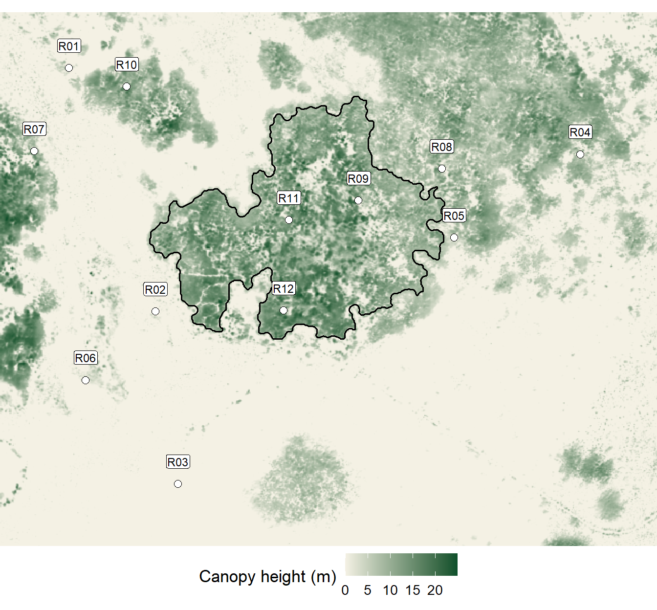
Canopy height around Kīpuka Puaulu. The black line is the kīpuka outline from Chapter 3; the circles are the twelve sample points.

The kīpuka stands out at once, a block of tall forest on open lava. So do the smaller patches of forest to the north and east, and the young ʻōhiʻa scattered across the flows. None of this is in the twelve points.

8.3 Four kinds of structure

The next step turns heights into a few classes of structure. Three choices go into it, and each one is written into the code where anyone can see it and change it.

1. Smooth the heights. Each cell takes the average height of the 25 by 25 meter square around it. A single tall tree on open lava shouldn’t make a patch of forest.
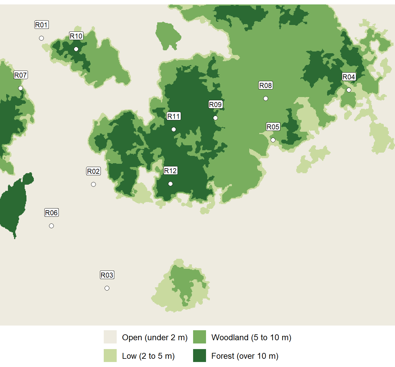
2. Break the heights into classes. Open (under 2 m), low (2 to 5 m), woodland (5 to 10 m), and forest (over 10 m). The 5 meter break is Fosberg’s line between scrub and forest.
3. Set a minimum mapping unit. Any patch smaller than 2 hectares joins its neighbors. That’s the scale of the map, the same kind of choice as the scale of a printed sheet. It’s close to the smallest patches on the 1974 map.

## step 1: smooth, averaging over a 25 m square (5 by 5 cells)
smooth <- focal(canopy, w = matrix(1, 5, 5) / 25, na.rm = TRUE)

## step 2: break the smoothed heights into four classes
breaks    <- c(-Inf, 2, 5, 10, Inf)
structure <- classify(smooth, cbind(breaks[-5], breaks[-1], 1:4))
class_names <- c("Open (under 2 m)", "Low (2 to 5 m)", "Woodland (5 to 10 m)", "Forest (over 10 m)")

## step 3: merge patches smaller than 2 hectares (800 cells of 25 square meters)
mmu_cells <- 20000 / 25
structure <- sieve(structure, threshold = mmu_cells, directions = 8)

## the classes as polygons, for drawing
structure_polys <- st_as_sf(as.polygons(structure))
names(structure_polys)[1] <- "class"
structure_polys <- mutate(structure_polys, class = factor(class_names[class], levels = class_names))

## draw them
ggplot() +
  geom_sf(data = structure_polys, aes(fill = class), color = NA) +
  geom_sf(data = releve_points, shape = 21, fill = "white", color = "black", size = 2.4) +
  geom_sf_label(data = releve_points, aes(label = releve), nudge_y = 110, size = 3,
                label.padding = unit(0.1, "lines"), fill = "white") +
  scale_fill_manual(values = c("#EEEBE0", "#C9DA9F", "#79AE5E", "#2B6A33"), name = NULL) +
  coord_sf(datum = NA, expand = FALSE) +
  theme_void(base_size = 13) +
  theme(legend.position = "bottom") +
  guides(fill = guide_legend(nrow = 2))

Four classes of canopy structure, with patches smaller than 2 hectares merged into their neighbors.

8.4 Tracing the kīpuka

Chapter 3 promised to show how the kīpuka outline was drawn. It uses the same smoothed heights, and it’s what someone would once have done by hand with an air photo and a pen.

## tall canopy: smoothed height over 8 m
tall <- ifel(smooth > 8, 1, NA)

## split the tall canopy into separate patches (touching edges, not corners)
tall_patches <- patches(tall, directions = 4)

## the kīpuka is the patch that holds point R11, in the heart of the forest
r11       <- vect(filter(releve_points, releve == "R11"))
kipuka_id <- extract(tall_patches, r11)[1, 2]
traced    <- st_as_sf(as.polygons(ifel(tall_patches == kipuka_id, 1, NA)))

## soften the stair-steps of the cells: 20 m out, then 20 m back in
traced <- st_buffer(st_buffer(traced, 20), -20)

## keep the largest piece, and only its outside ring (the glades are part of the kīpuka)
pieces <- st_cast(st_geometry(traced), "POLYGON")
largest <- pieces[[which.max(st_area(pieces))]]
traced  <- st_sfc(st_polygon(list(largest[[1]])), crs = 32605)

## compare with the outline used in Chapter 3
traced_ha     <- round(as.numeric(st_area(traced)) / 10000, 1)
chapter3_ha   <- round(as.numeric(st_area(kipuka)) / 10000, 1)
difference_ha <- round(as.numeric(st_area(st_sym_difference(traced, st_geometry(kipuka)))) / 10000, 2)

The traced outline covers 94.5 hectares. The one read from a file in Chapter 3 covers 94.5, and the two differ by 0.03 hectares, which is rounding in the stored heights. A few written rules replace the pen. Anyone who runs them gets the same kīpuka.

8.5 Tiles that follow the canopy

Now for the main step. The rule for a plain Voronoi map is that each place takes the category of the nearest point. The new rule adds a condition: each place takes the category of the nearest point in the same structure class. A point in a different kind of canopy counts as infinitely far away.

That’s the same move as in Chapter 7, where distance could be travel time. Here, distance is measured only within one kind of canopy. I’ll call the result a structure-constrained Voronoi map.

## the height and structure class at each point
point_vect <- vect(releve_points)
releves <- mutate(releves,
                  height_m = extract(canopy, point_vect)[, 2],
                  smooth_m = round(extract(smooth, point_vect)[, 2], 1),
                  class_id = extract(structure, point_vect)[, 2],
                  class    = class_names[class_id])

## show them
releves |>
  select(releve, vegetation, height_m, smooth_m, class) |>
  gt() |>
  cols_label(releve     = "Point",
             vegetation = "Vegetation (1974 map)",
             height_m   = "Canopy at the point (m)",
             smooth_m   = "Smoothed (m)",
             class      = "Structure class") |>
  tab_source_note(source_note = "Canopy height: Meta and World Resources Institute (2024). Vegetation: Mueller-Dombois and Fosberg (1974).")

Point	Vegetation (1974 map)	Canopy at the point (m)	Smoothed (m)	Structure class
R01	Koa-ʻōhiʻa forest	0.0	0.7	Open (under 2 m)
R02	ʻŌhiʻa scrub	0.0	0.6	Open (under 2 m)
R03	ʻŌhiʻa scrub	0.0	0.0	Open (under 2 m)
R04	ʻŌhiʻa forest	0.2	4.6	Low (2 to 5 m)
R05	ʻŌhiʻa forest	5.4	4.5	Low (2 to 5 m)
R06	ʻŌhiʻa scrub	3.0	2.4	Open (under 2 m)
R07	ʻŌhiʻa scrub	8.7	8.2	Woodland (5 to 10 m)
R08	Grass and savanna	2.2	5.0	Woodland (5 to 10 m)
R09	Kīpuka forest	7.6	8.0	Woodland (5 to 10 m)
R10	Koa-ʻōhiʻa forest	15.0	14.1	Forest (over 10 m)
R11	Kīpuka forest	9.2	10.4	Forest (over 10 m)
R12	Grass and savanna	14.7	11.6	Forest (over 10 m)
Canopy height: Meta and World Resources Institute (2024). Vegetation: Mueller-Dombois and Fosberg (1974).

The rule needs the distance from every cell to every point, then the nearest one, once with no condition and once within the same class.

## the center of every cell, and its structure class
cell_xy    <- xyFromCell(canopy, seq_len(ncell(canopy)))
cell_class <- values(structure)[, 1]

## distance from every cell to every point
distance <- sapply(seq_len(nrow(releves)), function(i) {
  sqrt(((cell_xy[, 1] - releves$easting[i])^2) + ((cell_xy[, 2] - releves$northing[i])^2))
})

## plain Voronoi: the nearest point wins
plain_winner <- max.col(-distance, ties.method = "first")

## structure-constrained: points in other classes are infinitely far away
same_class <- distance
same_class[outer(cell_class, releves$class_id, "!=")] <- Inf
constrained_winner <- max.col(-same_class, ties.method = "first")
## a class with no point in it stays blank
constrained_winner[!is.finite(same_class[cbind(seq_along(constrained_winner), constrained_winner)])] <- NA

## turn the winners into maps of vegetation type
type_names  <- names(veg_colors)
plain_map       <- setValues(rast(canopy), match(releves$vegetation[plain_winner], type_names))
constrained_map <- setValues(rast(canopy), match(releves$vegetation[constrained_winner], type_names))

## apply the 2 ha mapping unit to the finished map as well
constrained_map <- sieve(constrained_map, threshold = mmu_cells, directions = 8)

## how much of the study area changes type?
changed_pct <- round(100 * mean(values(plain_map)[, 1] != values(constrained_map)[, 1], na.rm = TRUE))

## a vegetation map as polygons, for drawing
map_polys <- function(veg_map) {
  polys <- st_as_sf(as.polygons(veg_map))
  names(polys)[1] <- "id"
  mutate(polys, vegetation = factor(type_names[id], levels = type_names))
}

## draw one vegetation map
draw_veg <- function(veg_map, title) {
  ggplot() +
    geom_sf(data = map_polys(veg_map), aes(fill = vegetation), color = NA) +
    geom_sf(data = kipuka, fill = NA, color = "black", linewidth = 0.6) +
    geom_sf(data = releve_points, shape = 21, fill = "white", color = "black", size = 2.2) +
    geom_sf_text(data = releve_points, aes(label = releve), nudge_y = 90, size = 3.4) +
    scale_fill_manual(values = veg_colors, breaks = names(veg_colors), name = NULL, drop = FALSE) +
    coord_sf(datum = NA, expand = FALSE) +
    labs(title = title, x = NULL, y = NULL) +
    theme_void(base_size = 13) +
    theme(plot.title = element_text(face = "bold"))
}

## stack the two, with one legend
(draw_veg(plain_map, "Plain Voronoi") / draw_veg(constrained_map, "Structure-constrained Voronoi")) +
  plot_layout(guides = "collect") +
  plot_annotation(theme = theme(legend.position = "bottom"))

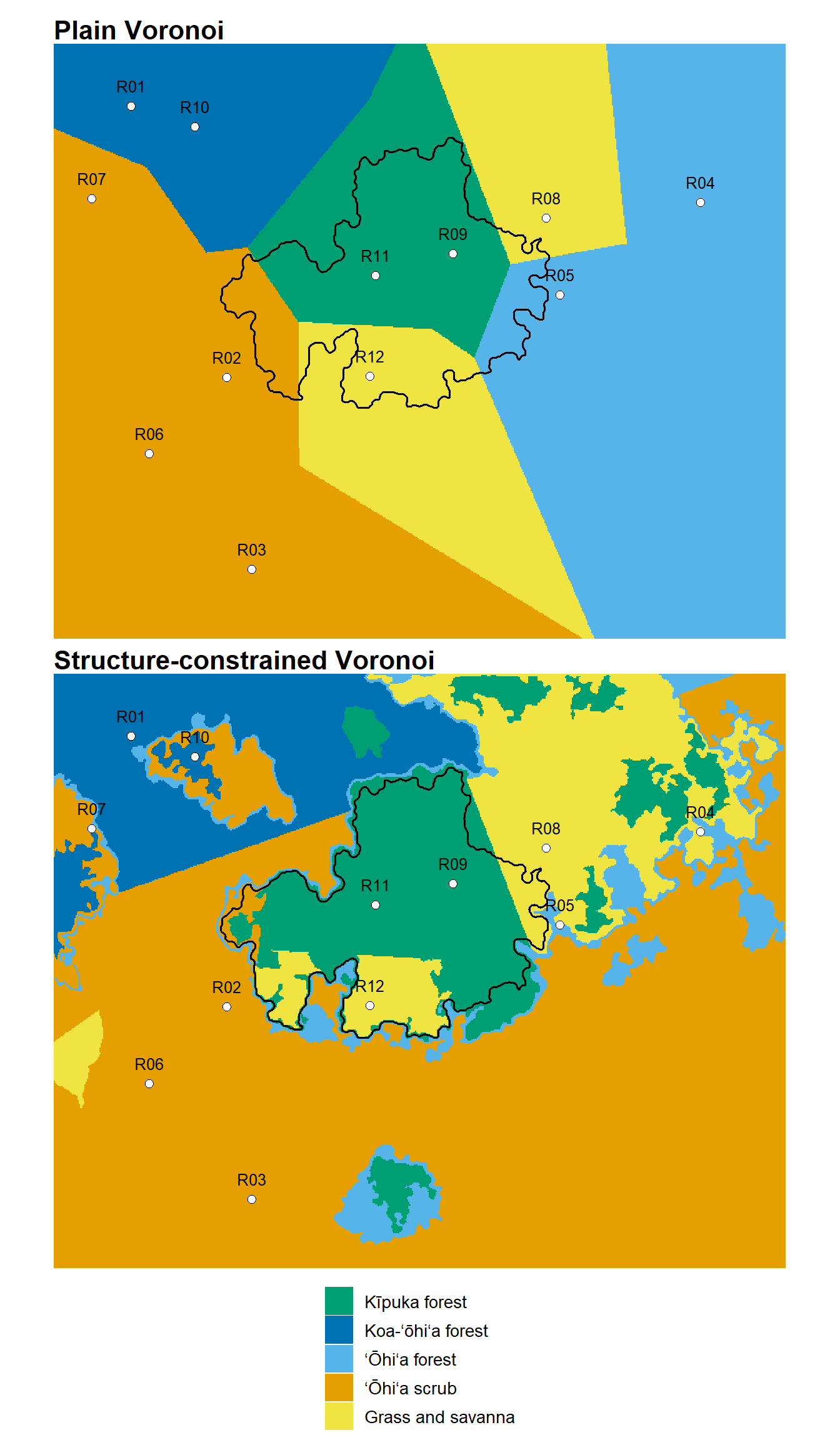
The same twelve points, mapped two ways. Top: plain Voronoi tiles. Bottom: structure-constrained tiles. The black line is the kīpuka outline.

The two maps disagree about the vegetation type of 51 percent of the study area. The plain map is a set of straight-sided tiles. The constrained map follows the canopy. The kīpuka forest now stops at the kīpuka’s edge instead of running out across the lava, the open flows take their labels from points on open ground, and the patches of taller forest to the north and east take theirs from points in tall forest. Some of the new edges look odd at first. The wide belt of woodland northeast of the kīpuka takes the grass and savanna label from R08, because R08 is the nearest point in that class. There’s history behind that, as the next section shows.

Even so, this is the turning point of this document. With the same twelve points, the boundaries now follow the edges of the canopy, which is where a person drawing a vegetation map would start, rather than halfway between two points.

8.6 When a label disagrees with the canopy

The constrained map also makes something visible that the plain map hides. Look at the table of points again.

Point R01 is labeled Koa-ʻōhiʻa forest on the 1974 map, but the canopy there today averages 0.7 meters. Point R12, inside the kīpuka, is labeled grass and savanna, but it stands under a canopy that averages 11.6 meters. That’s the point from Chapter 6 whose tile carried the grass label over the south end of the kīpuka.

In the plain map these disagreements don’t matter, because the plain map never looks at the ground. In the constrained map they matter a great deal. R12 is now one of the three points in the tallest class, so it hands the grass label to tall forest wherever it’s the nearest of the three.

The land has changed a great deal since the air photos behind the 1974 map were taken in 1954, and the change explains most of this.

• Cattle. Most of the Mauna Loa Strip was grazed by cattle for decades before it became part of the park. Kīpuka Puaulu itself was fenced before 1930, but cattle were allowed elsewhere in the Strip until 1940, came back during World War II, and weren’t finally removed until 1948 (Stone and Pratt 1994). The 1954 photos show the land six years later. Goats were fenced out in the 1970s, and pigs were removed in the mid-1980s.
• Koa. Once the cattle were gone, koa came up vigorously in the abandoned pastures around the kīpuka and formed a new forest canopy (Loh et al. 2007). Around the kīpuka, much of what the 1974 map calls grass and savanna now carries a tree canopy. That fits both R12 and the woodland belt around R08. It also means that some of the tall canopy inside today’s kīpuka outline was pasture when the photos were taken.
• Fire. On June 30, 2000, the Broomsedge Fire burned 1,008 acres of ʻōhiʻa woodland and koa forest east of the kīpuka. It came within 50 meters of the Kīpuka Puaulu Special Ecological Area before it was stopped (Loh et al. 2007). R04 and R05, east of the kīpuka, fall inside the burn, close to or perhaps inside the area where koa was planted afterward. They’re ʻōhiʻa forest on the 1974 map and stand in the low class today: a forest growing back. I’ve visited that area about once a year since the fire, and the regrowth has been remarkable. An earlier fire, in 1975, burned more than 2,000 acres upslope, between Kīpuka Kī and 5,000 feet (Stone and Pratt 1994).

So at R12 and R08, neither source is wrong. The map is mixing two dates: the names come from 1954, and the canopy comes from today. The disagreement is a record of seventy years of change.

R01 is less certain. It may have burned in the 1975 fire near Kīpuka Kī, but without a map of that burn there’s no way to be sure. The method can’t answer that. What it can do is flag the point, and that’s worth something on its own. A set of plot records checked against a canopy map is a quick way to find the ones that deserve a second look.

For a system that keeps changing, examining the data shouldn’t be the end point. Like any good science, the results should raise new questions. Here they do better than that: they turn a general sense that the land has changed into questions specific enough to answer.

• Did the 1975 fire reach R01? A map of that burn, or the park’s fire records, would settle it.
• How much of the tall canopy inside today’s kīpuka outline was pasture in 1954? The 1954 air photos could answer it, patch by patch.
• How fast is the Broomsedge burn growing back? A second canopy map from a later date, run through the same rules, would show how much of the low class has become woodland.
• Which points need a new relevé? R01, R12 and the points in the burn head the list.

Real relevés don’t have this problem in the same way. A field team records the structure and the species at the same spot on the same day. When their record disagrees with the canopy map, that’s news about the canopy map, or about change since the map was made.

8.7 What canopy height can’t do

Canopy height separates tall from short. It can’t separate one kind of tall forest from another. Where two points of different types sit in the same structure class, the boundary between their tiles is the old halfway line again. The clearest example is the long straight line across the open lava in the northwest. R01 and R02 are both on open ground, so the line between the koa-ʻōhiʻa label and the scrub label runs halfway between them, straight across a flow that looks the same on both sides. Inside the kīpuka, R11 and R12 are both in the tallest class, so the line between the kīpuka forest and the grass label runs straight across the forest. No canopy measure could move it. Only another point, or another kind of information about composition, could.

Some patches get their label from far away. A patch of woodland with no point in it still takes the type of the nearest woodland point, even if that point is across the study area.

## number the separate patches of each structure class
patch_id <- rast(canopy)
patch_id[] <- NA
offset <- 0
for (k in 1:4) {
  class_patches <- patches(ifel(structure == k, 1, NA), directions = 8)
  patch_id <- cover(patch_id, class_patches + offset)
  offset <- offset + global(class_patches, "max", na.rm = TRUE)[1, 1]
}

## patches that hold a point are sampled; the rest are extended from elsewhere
sampled_ids  <- unique(extract(patch_id, point_vect)[, 2])
sampled      <- values(patch_id)[, 1] %in% sampled_ids
extended_pct <- round(100 * mean(!sampled))
n_patches    <- offset

## the constrained map, as polygons, with the sampled patches marked
sampled_map   <- setValues(rast(canopy), as.integer(sampled))
sampled_polys <- st_as_sf(as.polygons(sampled_map))
names(sampled_polys)[1] <- "sampled"

## draw it: extended patches under a white veil
ggplot() +
  geom_sf(data = map_polys(constrained_map), aes(fill = vegetation), color = NA) +
  geom_sf(data = filter(sampled_polys, sampled == 0), fill = "white", alpha = 0.6, color = NA) +
  geom_sf(data = kipuka, fill = NA, color = "black", linewidth = 0.6) +
  geom_sf(data = releve_points, shape = 21, fill = "white", color = "black", size = 2.2) +
  geom_sf_label(data = releve_points, aes(label = releve), nudge_y = 110, size = 3,
                label.padding = unit(0.1, "lines"), fill = "white") +
  scale_fill_manual(values = veg_colors, breaks = names(veg_colors), name = NULL, drop = FALSE) +
  coord_sf(datum = NA, expand = FALSE) +
  theme_void(base_size = 13) +
  theme(legend.position = "bottom") +
  guides(fill = guide_legend(nrow = 2))

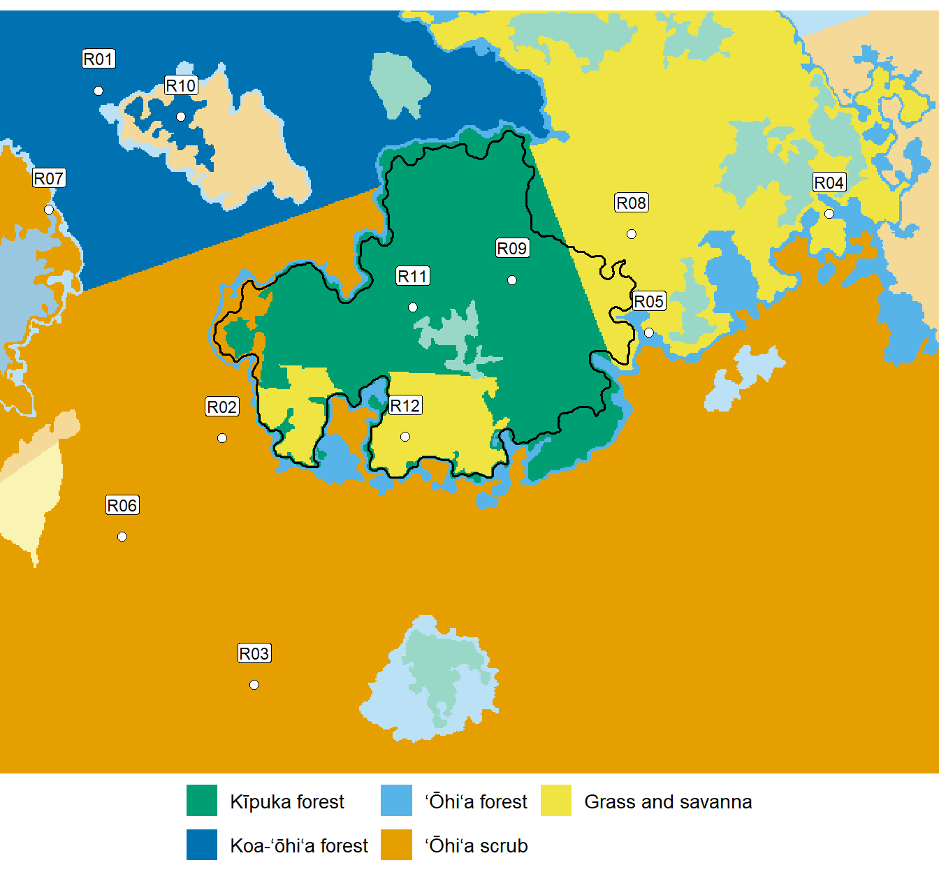
The structure-constrained map, with patches that hold no point shown faded. Their labels are extended from points in other patches of the same structure class.

The four structure classes break into 141 separate patches, and twelve points can sit in only a few of them. The patches with no point cover 11 percent of the study area. Their labels are a reasonable guess, and the map should say so. Fading them is one way.

A few more cautions belong with the method:

• The canopy map is a model. It’s made from images, not measured by lidar, so its edges are softer than the real ones and it can miss in places.
• The classes are choices. The smoothing, the height breaks and the 2 hectare unit are mine. They’re written down, so the map is reproducible. That’s not the same as objective, the distinction from Chapter 2.
• Smoothing and the mapping unit can move a point into a neighboring class. A point in a small opening can end up in the class of the forest around it, and a point in a patch smaller than 2 hectares takes the class of the patch that swallowed it. Compare the two height columns in the table above. A real relevé records its own structure, and that record should win.

8.8 What the points still decide

It’s worth being clear about the division of labor. The canopy decides where the boundaries go. The points still decide what the tiles are called. Twelve points can’t name more than twelve things, and a point with the wrong name spreads it just as far as before, only along better boundaries.

That division suits the way field work is actually done. Relevés are expensive, and the canopy map is free. If the canopy draws the lines, the relevés can go where they tell you the most: one or two in each kind of structure, rather than a grid dense enough to draw the edges by themselves. Chapter 9 tests that, by comparing these maps with the 1974 map and asking how many points it takes to get close.

NoteUseful?

Yes. This is where the tiles start to look like a vegetation map. A free canopy height map and a few written rules put the boundaries at the edges of the forest, where a person drawing the map would put them, and anyone can repeat the result. The points still carry the names, so the map is only as good as their labels, and one kind of tall forest still meets another on a straight line. The canopy map also turns out to be a quick check on the points themselves, and a record of how much the land has changed since the points were named.

The points say what grows there. The canopy says where it stops.

Arnold, D. B., and W. J. Milne. 1984. “The Use of Voronoi Tessellations in Processing Soil Survey Results.” IEEE Computer Graphics and Applications 4 (3): 22–28.

Loh, Rhonda, Sierra McDaniel, David Benitez, Matthew Schultz, David Palumbo, Alison Ainsworth, Kimberley Smith, Tim Tunison, and Maya Vaidya. 2007. “Rehabilitation of Seasonally Dry ʻŌhiʻa Woodlands and Mesic Koa Forest Following the Broomsedge Fire, Hawaiʻi Volcanoes National Park.” Technical Report 147. Honolulu: Pacific Cooperative Studies Unit, University of Hawaiʻi.

Stone, Charles P., and Linda W. Pratt. 1994. Hawaiʻi’s Plants and Animals: Biological Sketches of Hawaii Volcanoes National Park. Honolulu: Hawaii Natural History Association, National Park Service, and University of Hawaii Cooperative National Park Resources Studies Unit.

Tolan, Jamie, Hung-I Yang, Benjamin Nosarzewski, Guillaume Couairon, Huy V. Vo, John Brandt, Justine Spore, et al. 2024. “Very High Resolution Canopy Height Maps from RGB Imagery Using Self-Supervised Vision Transformer and Convolutional Decoder Trained on Aerial Lidar.” Remote Sensing of Environment 300: 113888. https://doi.org/10.1016/j.rse.2023.113888.