3  The Study Area

A Voronoi tessellation has no natural edge. The tiles around the outside of a group of points run on forever, because every place out there is still closer to one point than to the others. So before there’s a map, someone has to say where it stops.

That’s the one piece of outside information a plain Voronoi map accepts. My own notes from the start of this project put it this way: the mapped areas are based solely on the location of the points and the category of each point, and there’s an influence of the external border, but not any other information. This chapter is about that influence.

## --- Standard packages ---

## many useful functions, including read_csv() and ggplot()
library(tidyverse)
## formatted tables
library(gt)

## --- Specialized packages ---

## spatial data: points, polygons, and the Voronoi function
library(sf)

## --- Options and defaults ---

## suppress read_csv() column-type messages
options(readr.show_col_types = FALSE)

## the vegetation colors used throughout the document (Okabe-Ito palette)
veg_colors <- c("Kīpuka forest"     = "#009E73",
                "Koa-ʻōhiʻa forest" = "#0072B2",
                "ʻŌhiʻa forest"     = "#56B4E9",
                "ʻŌhiʻa scrub"      = "#E69F00",
                "Grass and savanna" = "#F0E442")

## the twelve sample points from Chapter 2, in UTM zone 5N
releves       <- read_csv("data/kipuka_puaulu_releves.csv")
releve_points <- st_as_sf(releves, coords = c("easting", "northing"), crs = 32605)

## the study area rectangle from Chapter 2
area_corners <- read_csv("data/kipuka_puaulu_study_area.csv")
study_box    <- st_bbox(c(xmin = area_corners$easting[1],
                          ymin = area_corners$northing[1],
                          xmax = area_corners$easting[2],
                          ymax = area_corners$northing[2]),
                        crs = st_crs(32605))
study_area   <- st_as_sfc(study_box)

3.1 Two kinds of study area

There are two ways to draw the border.

The first is a frame of convenience: a rectangle drawn around the points so the tiles have somewhere to stop. Arnold and Milne (1984) did this for the Greek soil survey. They chose a rectangular window that enclosed all their sample points. The rectangle in Chapter 2 is the same kind of frame. It doesn’t claim anything about the land.

The second is a boundary that means something. Johnston and her colleagues (1996) mapped a wetland, so they traced the wetland’s edge from their airborne video and clipped the tiles to it. A park boundary, a lava flow, the edge of a kīpuka, or an ahupuaʻa, running from the uplands to the sea, are all boundaries of this kind. Each one says that the area inside is a unit and that what lies outside belongs to something else. Ahupuaʻa were important boundaries in Hawaiian culture, and they matter still. Today we’re marking them again in our neighborhoods.

The two kinds behave differently, and it’s worth seeing how.

3.2 Edge tiles

In a frame of convenience, the tiles along the border have a problem. Their size depends on where the border was drawn, not on the vegetation.

The quickest way to see it is to move the border. The code below builds the tiles twice: once in the Chapter 2 rectangle, and once in a rectangle 500 meters larger on every side. Then it compares the area of each tile.

## a function for the three tile-building steps from Chapter 2
make_tiles <- function(points, frame) {
  ## build the tiles around all the points
  tiles_all <- st_voronoi(st_union(points), envelope = frame)
  ## split the result into separate polygons
  tiles <- st_collection_extract(tiles_all)
  ## trim the tiles to the frame
  tiles <- st_intersection(tiles, frame)
  ## attach each tile to the point inside it
  tiles <- st_sf(geometry = tiles)
  st_join(tiles, points)
}

## the larger frame: 500 m added on every side
larger_box  <- st_bbox(c(xmin = area_corners$easting[1]  - 500,
                         ymin = area_corners$northing[1] - 500,
                         xmax = area_corners$easting[2]  + 500,
                         ymax = area_corners$northing[2] + 500),
                       crs = st_crs(32605))
larger_area <- st_as_sfc(larger_box)

## tiles in each frame
tiles_small <- make_tiles(releve_points, study_area)
tiles_large <- make_tiles(releve_points, larger_area)

## which tiles touch the border of the original frame?
frame_edge <- st_boundary(study_area)
tiles_small <- mutate(tiles_small, edge = lengths(st_intersects(geometry, frame_edge)) > 0)

## tile areas in hectares, for each frame
areas_small <- tibble(releve   = tiles_small$releve,
                      edge     = tiles_small$edge,
                      small_ha = as.numeric(st_area(tiles_small)) / 10000)
areas_large <- tibble(releve   = tiles_large$releve,
                      large_ha = as.numeric(st_area(tiles_large)) / 10000)

## put the two side by side and compute the change
area_compare <- left_join(areas_small, areas_large, by = "releve")
area_compare <- mutate(area_compare,
                       change_pct = round(100 * ((large_ha - small_ha) / small_ha)),
                       small_ha   = round(small_ha, 1),
                       large_ha   = round(large_ha, 1))
area_compare <- arrange(area_compare, releve)

## show it
area_compare |>
  gt() |>
  cols_label(releve     = "Point",
             edge       = "Edge tile?",
             small_ha   = "Area, original frame (ha)",
             large_ha   = "Area, larger frame (ha)",
             change_pct = "Change (%)")

Point	Edge tile?	Area, original frame (ha)	Area, larger frame (ha)	Change (%)
R01	TRUE	23.1	94.3	308
R02	FALSE	51.8	51.8	0
R03	TRUE	94.2	235.5	150
R04	TRUE	101.2	282.2	179
R05	TRUE	159.2	230.4	45
R06	TRUE	63.2	137.4	117
R07	TRUE	39.0	93.7	140
R08	TRUE	60.4	99.3	64
R09	TRUE	44.0	45.0	2
R10	TRUE	62.0	108.5	75
R11	FALSE	44.8	44.8	0
R12	TRUE	88.9	89.0	0

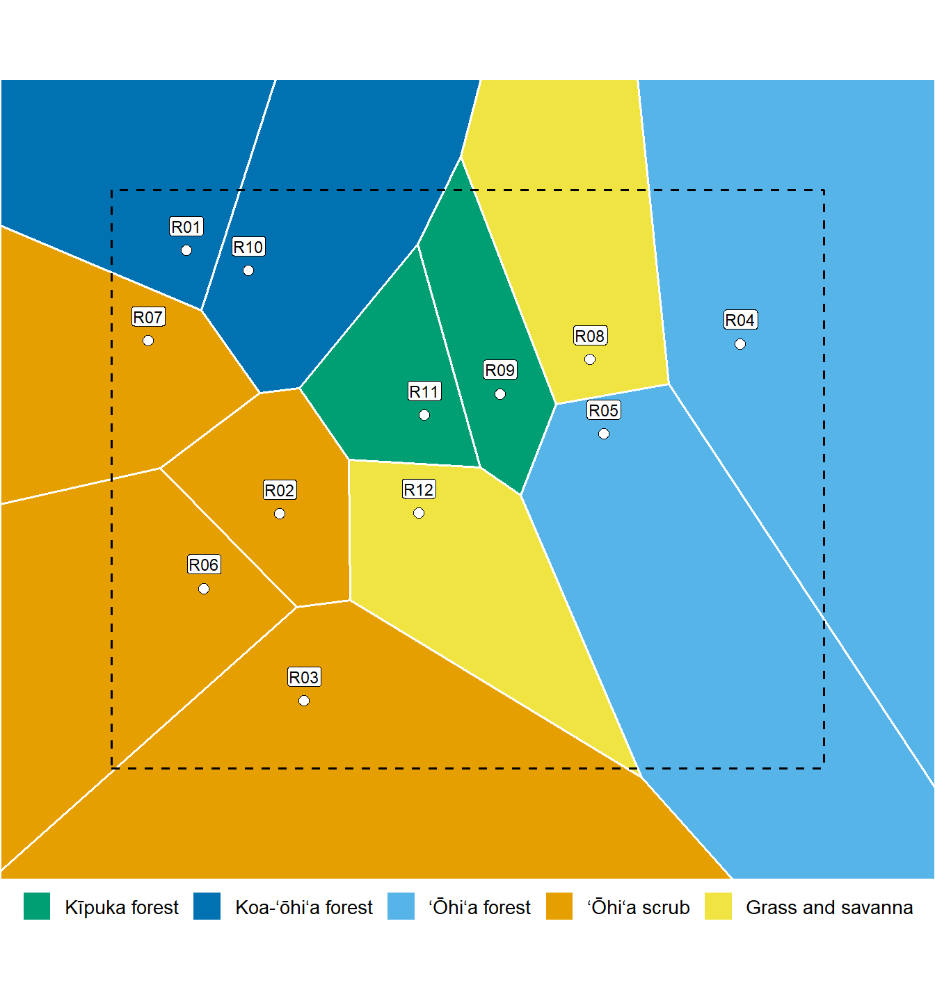
10 of the twelve tiles touch the border, and only 2 don’t. When the frame grows, 9 tiles change size, and every one of them is an edge tile. The interior tiles stay exactly as they were, because their edges are set by their neighbors on every side.

## draw the tiles in the larger frame, with the original frame dashed
ggplot() +
  geom_sf(data = tiles_large, aes(fill = vegetation), color = "white", linewidth = 0.6) +
  geom_sf(data = study_area, fill = NA, color = "black", linetype = "dashed", linewidth = 0.7) +
  geom_sf(data = releve_points, shape = 21, fill = "white", color = "black", size = 2.4) +
  geom_sf_label(data = releve_points, aes(label = releve), nudge_y = 110, size = 3,
                label.padding = unit(0.1, "lines"), fill = "white") +
  scale_fill_manual(values = veg_colors, breaks = names(veg_colors), name = NULL) +
  coord_sf(datum = NA, expand = FALSE) +
  theme_void(base_size = 13) +
  theme(legend.position = "bottom")

Tiles in the larger frame. The dashed line is the original frame. Every tile that reaches the dashed line grew when the frame grew; the others didn’t change.

So the area of an edge tile tells you where the border was drawn. It doesn’t tell you about the vegetation. Arnold and Milne ran into the same thing. They wrote that there are two occasions when sample points “appear to have undue influence” on the tessellation: when they lie near the edges of the map sheet, and when they lie near built-up areas and other unsurveyed regions.

Three habits keep the problem in hand:

• Stop the frame where the sampling stops. A frame drawn well beyond the last points hands the extra ground to whichever points happen to be on the outside.
• Sample past the area you care about, then clip. Points outside the area of interest give the tiles inside it real neighbors.
• Report edge tiles separately. Any statistic that uses tile area, such as the area of each vegetation type in Chapter 2, should say how much of it comes from edge tiles.

3.3 A boundary that means something

Kīpuka Puaulu is a good example of a real boundary. It’s an island of old forest, and the lava flows around it are younger and much more open. The edge between the two is sharp, and it’s easy to see from the air.

The outline below was traced from a map of canopy height, where the forest stands more than 8 meters tall. It’s the line someone would once have traced by hand from an air photo; here the canopy map does the tracing. Chapter 8 shows how. For now it’s simply a boundary, read from a file.

## the outline of the kīpuka
kipuka <- st_read("data/kipuka_puaulu_outline.geojson", quiet = TRUE)

## which sample points fall inside it?
inside <- lengths(st_intersects(releve_points, kipuka)) > 0
points_inside <- releve_points[inside, ]

## show them
points_inside |>
  st_drop_geometry() |>
  gt() |>
  tab_header(title = "Sample points inside the kīpuka outline")

Sample points inside the kīpuka outline
releve	vegetation
R09	Kīpuka forest
R11	Kīpuka forest
R12	Grass and savanna

The outline encloses about 95 hectares, and 3 of the twelve points fall inside it. There are two ways to map the kīpuka from here.

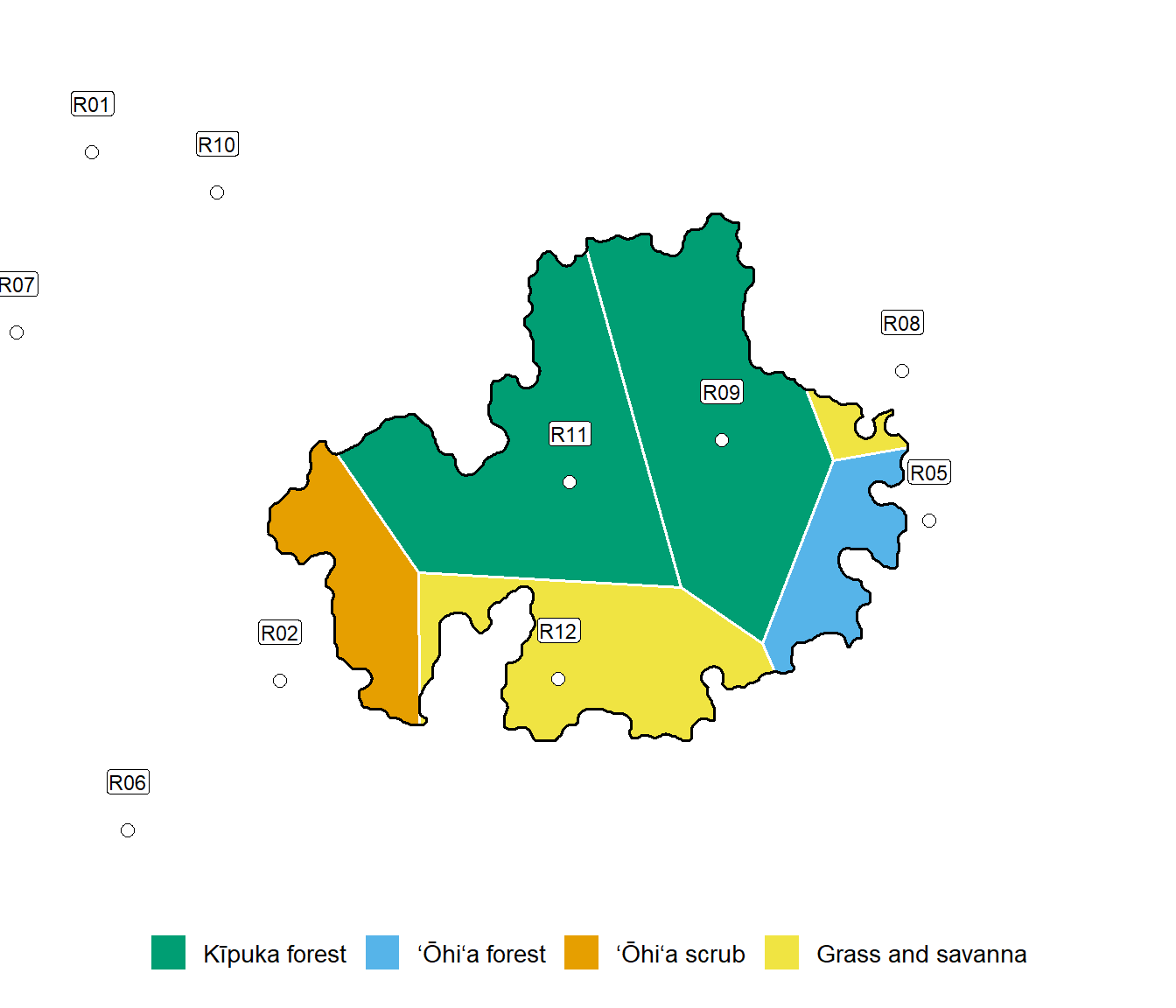
Tessellate everything, then clip. Build the tiles from all twelve points, exactly as before, and cut them to the kīpuka outline. Points outside the kīpuka still claim part of it, wherever they happen to be nearer than any point inside.

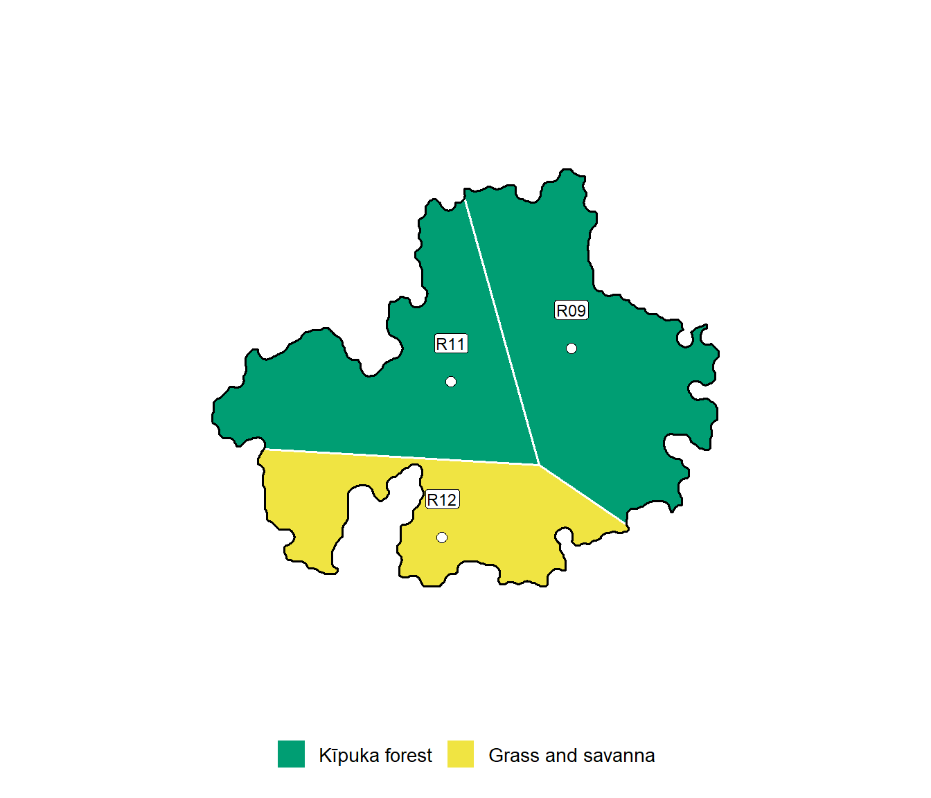
Tessellate only what’s inside. Use only the points inside the kīpuka, and let their tiles fill it. Points on the lava outside have no say.

## way 1: tiles from all twelve points, clipped to the kīpuka
all_then_clip <- st_intersection(tiles_small, st_geometry(kipuka))

## way 2: tiles from the inside points only, clipped to the kīpuka
kipuka_frame  <- st_as_sfc(st_bbox(kipuka))
inside_only   <- make_tiles(points_inside, kipuka_frame)
inside_only   <- st_intersection(inside_only, st_geometry(kipuka))

## how much of the kīpuka does each point claim under way 1?
claims <- tibble(releve     = all_then_clip$releve,
                 vegetation = all_then_clip$vegetation,
                 point_is   = if_else(all_then_clip$releve %in% points_inside$releve,
                                      "inside", "outside"),
                 area_ha    = round(as.numeric(st_area(all_then_clip)) / 10000, 1))
claims <- arrange(claims, desc(area_ha))

## show it
claims |>
  gt() |>
  tab_header(title = "Tessellate everything, then clip: who claims the kīpuka?")

Tessellate everything, then clip: who claims the kīpuka?
releve	vegetation	point_is	area_ha
R09	Kīpuka forest	inside	28.6
R11	Kīpuka forest	inside	28.3
R12	Grass and savanna	inside	17.8
R02	ʻŌhiʻa scrub	outside	10.5
R05	ʻŌhiʻa forest	outside	7.6
R08	Grass and savanna	outside	1.6

Under the first way, points outside the kīpuka claim about 21 percent of it. Their tiles reach across the forest edge and label old forest with whatever was recorded out on the lava.

## way 1
ggplot() +
  geom_sf(data = all_then_clip, aes(fill = vegetation), color = "white", linewidth = 0.6) +
  geom_sf(data = kipuka, fill = NA, color = "black", linewidth = 0.7) +
  geom_sf(data = releve_points, shape = 21, fill = "white", color = "black", size = 2.4) +
  geom_sf_label(data = releve_points, aes(label = releve), nudge_y = 110, size = 3,
                label.padding = unit(0.1, "lines"), fill = "white") +
  scale_fill_manual(values = veg_colors, breaks = names(veg_colors), name = NULL) +
  coord_sf(datum = NA, xlim = st_bbox(kipuka)[c(1, 3)] + c(-600, 600),
           ylim = st_bbox(kipuka)[c(2, 4)] + c(-400, 400), expand = FALSE) +
  theme_void(base_size = 13) +
  theme(legend.position = "bottom")

Tessellate everything, then clip. Points outside the kīpuka (hollow circles outside the outline) still claim parts of it.

## way 2
ggplot() +
  geom_sf(data = inside_only, aes(fill = vegetation), color = "white", linewidth = 0.6) +
  geom_sf(data = kipuka, fill = NA, color = "black", linewidth = 0.7) +
  geom_sf(data = points_inside, shape = 21, fill = "white", color = "black", size = 2.4) +
  geom_sf_label(data = points_inside, aes(label = releve), nudge_y = 110, size = 3,
                label.padding = unit(0.1, "lines"), fill = "white") +
  scale_fill_manual(values = veg_colors, breaks = names(veg_colors), name = NULL) +
  coord_sf(datum = NA, xlim = st_bbox(kipuka)[c(1, 3)] + c(-600, 600),
           ylim = st_bbox(kipuka)[c(2, 4)] + c(-400, 400), expand = FALSE) +
  theme_void(base_size = 13) +
  theme(legend.position = "bottom")

Tessellate only what’s inside. The kīpuka is divided among its own points.

Which way is right depends on what the boundary means. If it’s only a frame, the first way is fine. If it’s a real edge, the second way says so. Nothing on the young lava tells you anything about the old forest, so the lava points shouldn’t have a vote inside it.

That’s a small step with a large consequence. The boundary is information the points don’t carry, and using it changes the map. Chapter 8 takes the same idea much further, using canopy height to supply boundaries everywhere, not only around the edge of the study area.

NoteUseful?

Yes, with one discipline. Say where the border came from. If it’s a frame of convenience, keep it close to the sampling and report the edge tiles separately. If it’s a real boundary, such as a wetland edge, a kīpuka or an ahupuaʻa, decide whether points outside it should count, and say which you chose.

Inside the border, the points decide. Where the border goes is up to you.

Arnold, D. B., and W. J. Milne. 1984. “The Use of Voronoi Tessellations in Processing Soil Survey Results.” IEEE Computer Graphics and Applications 4 (3): 22–28.

Johnston, Carol A., Carol A. Sersland, John Bonde, Deb Pomroy-Petry, and Paul Meysembourg. 1996. “Constructing Detailed Vegetation Databases from Field Data and Airborne Videography.” In Proceedings of the Third International Conference/Workshop on Integrating GIS and Environmental Modeling, Santa Fe, New Mexico. Santa Barbara, California: National Center for Geographic Information and Analysis. http://www.ncgia.ucsb.edu/SANTA_FE_CD-ROM/sf_papers/johnston_carol/paper2.html.