9  Good Enough?

Chapter 1 set two maps side by side and asked a question: can Voronoi tessellations make maps with the border complexity of hand-drawn vegetation maps? It’s time to answer it.

The hand-drawn map is the obvious yardstick. Fosberg drew it from air photos taken in 1954, Mueller-Dombois checked it on the ground in 1965, and it was published in 1974 (Mueller-Dombois and Fosberg 1974). But Chapter 8 showed that it can’t be treated as the truth. Cattle left the Mauna Loa Strip in 1948, koa has grown up in the old pastures, and fire has burned the woodland east of the kīpuka. The 1974 map is a careful record of a landscape that has since changed.

Johnston et al. (1996) took the right attitude. They compared their Thiessen polygon map with a map made from airborne video and concluded that “one cannot be thought of as more ‘correct’ than the other.” That’s the spirit of this chapter. The 1974 map is a benchmark with a date on it, not an answer key.

## --- Standard packages ---

## many useful functions, including read_csv() and ggplot()
library(tidyverse)
## formatted tables
library(gt)
## stacking figures
library(patchwork)

## --- Specialized packages ---

## spatial vector data: points, polygons
library(sf)
## spatial raster data: grids of cells
library(terra)

## --- Options and defaults ---

## suppress read_csv() column-type messages
options(readr.show_col_types = FALSE)

## the vegetation colors used throughout the document (Okabe-Ito palette)
veg_colors <- c("Kīpuka forest"     = "#009E73",
                "Koa-ʻōhiʻa forest" = "#0072B2",
                "ʻŌhiʻa forest"     = "#56B4E9",
                "ʻŌhiʻa scrub"      = "#E69F00",
                "Grass and savanna" = "#F0E442")
type_names <- names(veg_colors)

## the twelve sample points, the kīpuka outline and the canopy map
releves       <- read_csv("data/kipuka_puaulu_releves.csv")
releve_points <- st_as_sf(releves, coords = c("easting", "northing"), crs = 32605)
kipuka        <- st_transform(st_read("data/kipuka_puaulu_outline.geojson", quiet = TRUE), 32605)
canopy        <- rast("data/kipuka_puaulu_canopy_height.tif")

## the structure classes from Chapter 8: smooth, break at 2, 5 and 10 m, 2 ha mapping unit
mmu_cells   <- 20000 / 25
smooth      <- focal(canopy, w = matrix(1, 5, 5) / 25, na.rm = TRUE)
structure   <- classify(smooth, cbind(c(-Inf, 2, 5, 10), c(2, 5, 10, Inf), 1:4))
structure   <- sieve(structure, threshold = mmu_cells, directions = 8)
class_names <- c("Open", "Low", "Woodland", "Forest")

9.1 The 1974 map as data

To compare maps cell by cell, the hand-drawn map has to become data. The vegetation overlays of sheets 12 and 13 were cut from the scanned report, fitted to the corner marks of each sheet, and traced into regions. Each region was coded by its map symbol and grouped into the same five types the sample points use. The sheets were drawn on the Old Hawaiian Datum, so the result was shifted about 285 meters east and 345 meters south to sit on today’s coordinates. Kīpuka Kī, in the northwest corner, is left blank because its outline is broken in the scan. The script that makes the file is in the project’s R folder.

The test of the fitting is whether the old lines land on today’s ground. They do. The edge of the kīpuka on the 1974 map sits on the edge of the tall canopy in Chapter 8.

## the 1974 map on the study-area grid (5 m cells): one vegetation class per cell
mdf1974      <- rast("data/mdf1974_classes.tif")
mdf1974_list <- read_csv("data/mdf1974_classes.csv")

## the 1974 types, as numbers matching type_names
mdf_values <- values(mdf1974)[, 1]
coded      <- !is.na(mdf_values)

9.2 Rebuilding the two maps

The two maps from Chapter 8 are rebuilt here from the same twelve points, with one change. Each point now takes the 1974 type at its own location, which is what the points have carried since Chapter 2. So any disagreement below comes from the method, the twelve points, or the years, not from mislabeled points.

## the center and structure class of every cell
cell_xy    <- xyFromCell(canopy, seq_len(ncell(canopy)))
cell_class <- values(structure)[, 1]

## a function that assigns every cell to its nearest point, with or without the structure rule
nearest_type <- function(px, py, type, point_class, constrained) {
  best <- rep(Inf, nrow(cell_xy))
  out  <- rep(NA_integer_, nrow(cell_xy))
  for (i in seq_along(px)) {
    ## squared distance from every cell to point i
    d <- ((cell_xy[, 1] - px[i])^2) + ((cell_xy[, 2] - py[i])^2)
    ## under the structure rule, points in other classes are out of reach
    if (constrained) d[cell_class != point_class[i]] <- Inf
    ## keep point i wherever it's nearer than anything found so far
    closer <- d < best
    best[closer] <- d[closer]
    out[closer]  <- type[i]
  }
  out
}

## the type and structure class at each of the twelve points
point_vect  <- vect(releve_points)
point_type  <- match(releves$vegetation, type_names)
point_class <- terra::extract(structure, point_vect)[, 2]

## plain Voronoi and structure-constrained Voronoi (with the 2 ha unit), as in Chapter 8
plain_values <- nearest_type(releves$easting, releves$northing, point_type, point_class, FALSE)
constrained_values <- nearest_type(releves$easting, releves$northing, point_type, point_class, TRUE)
constrained_values <- values(sieve(setValues(rast(canopy), constrained_values),
                                   threshold = mmu_cells, directions = 8))[, 1]

9.3 Two ways to agree

There are two ways to ask whether two vegetation maps agree.

Area agreement asks what share of the ground gets the same type on both maps. It’s the usual measure, and it’s the one Johnston reported.

Boundary agreement asks whether the lines fall in the same places. It’s closer to the question in Chapter 1, which was about borders. Two numbers describe it. The first is the share of the 1974 boundary that lies within 50 meters of a boundary on our map: how much of Fosberg’s line work we found. The second runs the other way: the share of our boundary that lies within 50 meters of a 1974 line. Fifty meters is one millimeter on the printed 1:52,000 map, about as close as a careful hand and the fitting of the old sheets can be trusted.

## area agreement: share of coded cells with the same type
area_agree <- function(v) mean(!is.na(v[coded]) & v[coded] == mdf_values[coded])

## boundary cells of a map (cells whose neighbor has a different type)
edges_of <- function(v) boundaries(setValues(rast(canopy), v), classes = TRUE, directions = 4)

## the 1974 boundary, and the distance from every cell to it
mdf_edges    <- edges_of(ifelse(coded, mdf_values, NA))
mdf_on_edge  <- values(mdf_edges)[, 1] == 1
to_mdf_edge  <- values(distance(classify(mdf_edges, cbind(0, NA))))[, 1]

## boundary agreement for one map
boundary_agree <- function(v) {
  map_edges <- edges_of(v)
  on_edge   <- values(map_edges)[, 1] == 1
  to_edge   <- values(distance(classify(map_edges, cbind(0, NA))))[, 1]
  tibble(found   = mean(to_edge[which(mdf_on_edge)] <= 50),
         on_1974 = mean(to_mdf_edge[which(on_edge & coded)] <= 50),
         km      = sum(on_edge, na.rm = TRUE) * 5 / 1000)
}

## the table
agreement <- bind_rows(
  tibble(map = "Plain Voronoi", area = area_agree(plain_values), boundary_agree(plain_values)),
  tibble(map = "Structure-constrained", area = area_agree(constrained_values), boundary_agree(constrained_values)))
mdf_km <- sum(mdf_on_edge, na.rm = TRUE) * 5 / 1000

## show it
agreement |>
  gt() |>
  cols_label(map     = "Map (twelve points)",
             area    = "Same type (% of area)",
             found   = "1974 boundary found (%)",
             on_1974 = "Our boundary on a 1974 line (%)",
             km      = "Boundary drawn (km)") |>
  fmt_percent(columns = c(area, found, on_1974), decimals = 0) |>
  fmt_number(columns = km, decimals = 0) |>
  tab_source_note(source_note = paste0("Boundaries within 50 m count as found. The 1974 map has about ",
                                       round(mdf_km), " km of boundary in the study area."))

Map (twelve points)	Same type (% of area)	1974 boundary found (%)	Our boundary on a 1974 line (%)	Boundary drawn (km)
Plain Voronoi	45%	17%	46%	18
Structure-constrained	56%	58%	54%	107
Boundaries within 50 m count as found. The 1974 map has about 51 km of boundary in the study area.

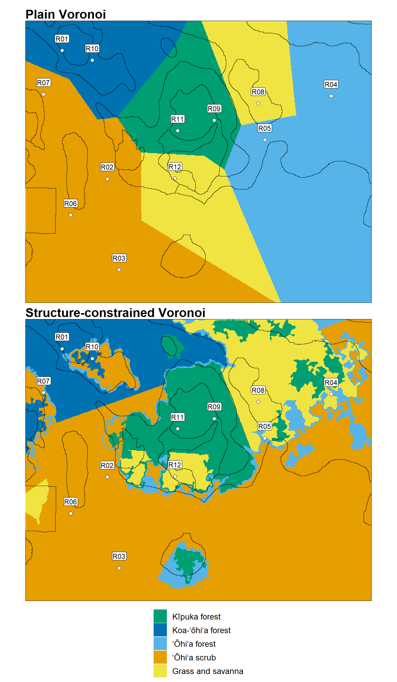
The two numbers tell different stories. Area agreement rises from 45 to 56 percent. That’s a real gain, but a modest one. Boundary agreement changes much more. The plain map finds 17 percent of the 1974 boundary. The constrained map finds 58 percent.

## the 1974 boundaries as lines
mdf_polys <- st_as_sf(as.polygons(mdf1974))
mdf_lines <- st_boundary(mdf_polys)

## a map of types as polygons
type_polys <- function(v) {
  polys <- st_as_sf(as.polygons(setValues(rast(canopy), v)))
  names(polys)[1] <- "id"
  mutate(polys, vegetation = factor(type_names[id], levels = type_names))
}

## draw one map with the 1974 lines over it
draw_with_lines <- function(v, title) {
  ggplot() +
    geom_sf(data = type_polys(v), aes(fill = vegetation), color = NA) +
    geom_sf(data = mdf_lines, color = "black", linewidth = 0.35) +
    geom_sf(data = releve_points, shape = 21, fill = "white", color = "black", size = 2) +
    geom_sf_label(data = releve_points, aes(label = releve), nudge_y = 110, size = 3,
                  label.padding = unit(0.1, "lines"), fill = "white") +
    scale_fill_manual(values = veg_colors, breaks = type_names, name = NULL, drop = FALSE) +
    coord_sf(datum = NA, expand = FALSE) +
    labs(title = title, x = NULL, y = NULL) +
    theme_void(base_size = 13) +
    theme(plot.title = element_text(face = "bold"))
}

## stack the two, with one legend
(draw_with_lines(plain_values, "Plain Voronoi") /
   draw_with_lines(constrained_values, "Structure-constrained Voronoi")) +
  plot_layout(guides = "collect") +
  plot_annotation(theme = theme(legend.position = "bottom"))

The 1974 boundaries (black lines) over the two maps made from twelve points. Top: plain Voronoi. Bottom: structure-constrained Voronoi. The rectangle on the left edge is Kīpuka Kī, left blank.

The constrained map also draws far more boundary than Fosberg did: about 107 kilometers against his 51. Only 54 percent of it lies on a 1974 line. Some of the extra is detail he chose not to draw. His savanna and mosaic units lumped small stands of trees and open ground together, and the canopy map splits them apart. The 2 hectare unit from Chapter 8 already trims the smallest pieces; a larger unit would trim more, at the cost of finding fewer of his lines. That’s a choice of scale, not a correction. The rest of the extra boundary is change, which comes next.

9.4 How many points?

Twelve points is a small number, and the comparison above could be luck. A fair test repeats it with different points and different numbers of points.

The test below places points at random, from 6 to 192 of them, twenty times at each number. Each point takes the 1974 type at its location. Then it builds both maps and measures area agreement. It does this two ways. In the first, the points fall anywhere. In the second, they’re stratified: split evenly among the four structure classes, the way a field team might place relevés after looking at the canopy map. The code takes several minutes to run.

## the numbers of points to try, and the number of tries at each
point_counts <- c(6, 12, 24, 48, 96, 192)
tries        <- 20

## repeat the comparison with new points
set.seed(20260926)
trials <- list()
for (n in point_counts) {
  for (try in seq_len(tries)) {
    for (design in c("Random", "Stratified by structure")) {
      ## choose the cells that hold the points
      if (design == "Random") {
        chosen <- sample(which(coded), n)
      } else {
        chosen <- unlist(lapply(1:4, function(k) {
          in_class <- which(cell_class == k & coded)
          in_class[sample.int(length(in_class), ceiling(n / 4))]
        }))[1:n]
      }
      ## each point takes the 1974 type and the structure class at its cell
      px <- cell_xy[chosen, 1]
      py <- cell_xy[chosen, 2]
      pt <- mdf_values[chosen]
      pc <- cell_class[chosen]
      ## the two maps
      plain       <- nearest_type(px, py, pt, pc, FALSE)
      constrained <- nearest_type(px, py, pt, pc, TRUE)
      constrained <- values(sieve(setValues(rast(canopy), constrained), threshold = mmu_cells, directions = 8))[, 1]
      ## record the area agreement of each
      trials[[length(trials) + 1]] <- tibble(points = n, try = try, design = design,
                                            Plain = area_agree(plain),
                                            `Structure-constrained` = area_agree(constrained))
    }
  }
}
trials <- bind_rows(trials)

## long form, and a summary for each number of points
trials_long <- pivot_longer(trials, c(Plain, `Structure-constrained`), names_to = "map", values_to = "agreement")
curve <- summarise(group_by(trials_long, design, map, points),
                   median = median(agreement),
                   low    = quantile(agreement, 0.25),
                   high   = quantile(agreement, 0.75),
                   .groups = "drop")

## draw it: one panel per design, stacked
ggplot(curve, aes(x = points, y = median, color = map, fill = map)) +
  geom_ribbon(aes(ymin = low, ymax = high), alpha = 0.2, color = NA) +
  geom_line(linewidth = 0.9) +
  geom_point(size = 2) +
  facet_wrap(~ design, ncol = 1) +
  scale_x_log10(breaks = point_counts) +
  scale_y_continuous(labels = scales::percent) +
  scale_color_manual(values = c("Plain" = "#999999", "Structure-constrained" = "#009E73"), name = NULL) +
  scale_fill_manual(values = c("Plain" = "#999999", "Structure-constrained" = "#009E73"), name = NULL) +
  labs(x = "Number of points", y = "Same type as the 1974 map") +
  theme_minimal(base_size = 13) +
  theme(legend.position = "bottom", panel.grid.minor = element_blank())

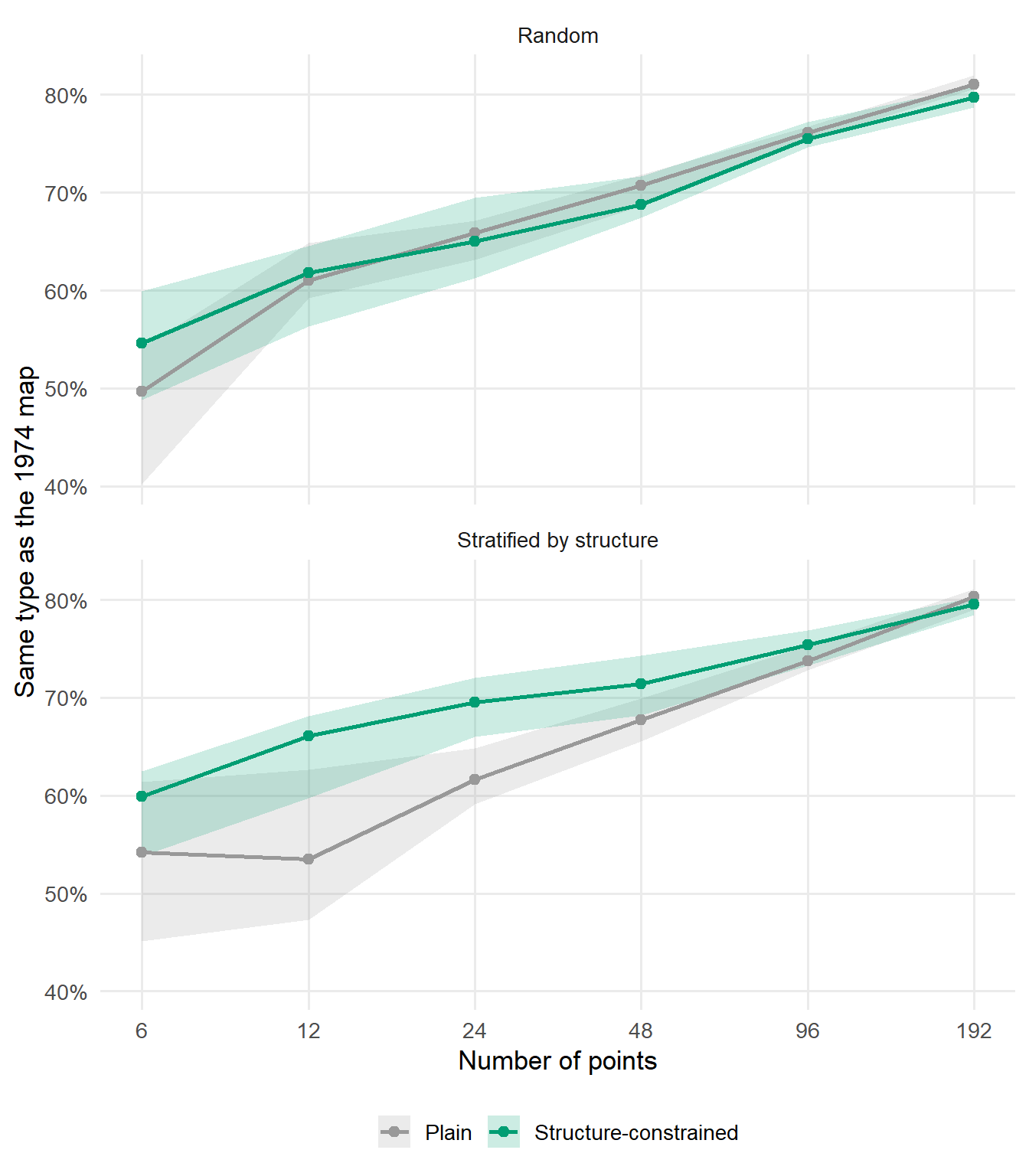
Area agreement with the 1974 map as the number of points grows. Lines join the medians of twenty tries; bands span the middle half of the tries.

The two panels tell different stories. With random points, the canopy makes little difference. The two lines run together, and from about 24 points on the plain map does as well or a little better.

With points stratified by structure, the constrained map leads clearly while the points are few: 66 percent against 53 with twelve points, and 70 against 62 with 24. The lead shrinks as points are added, and by 96 the two lines meet. With that many points, the points find the edges on their own.

That’s the part that matters for field work. Twelve stratified points with the canopy do about as well as 24 random points with plain tiles (66 percent). Put simply, the canopy map does the work of about half the relevés, when they’re few and placed with the canopy in mind.

The stratified plain map shows why placement alone isn’t the answer. Spreading the points evenly across the four structure classes puts too few on the open lava, which covers most of the study area, so plain tiles from those points do worse than random ones. The structure rule fixes that, because it keeps each point’s name inside its own class.

The twelve points used in this document turn out to be a below-average draw. Their constrained map agrees on 56 percent of the area, and 16 of the twenty stratified tries with twelve points did better. The conclusions don’t rest on them.

9.5 How much is change?

Some of the disagreement isn’t the method’s fault. The land has changed, and a map made from today’s canopy can’t agree with a map of 1954 where the vegetation itself is different. The table below sets the two dates against each other. Each row is a 1974 type; the columns show what the canopy is like on that ground today.

## 1974 type against today's structure class, as a share of each 1974 type
then_now <- tibble(vegetation = type_names[mdf_values[coded]],
                   today      = class_names[cell_class[coded]])
then_now <- count(then_now, vegetation, today)
then_now <- mutate(group_by(then_now, vegetation), share = n / sum(n))
then_now <- pivot_wider(ungroup(then_now), id_cols = vegetation, names_from = today,
                        values_from = share, values_fill = 0)
then_now <- then_now[match(type_names, then_now$vegetation), c("vegetation", class_names)]

## show it
then_now |>
  gt() |>
  cols_label(vegetation = "1974 type") |>
  tab_spanner(label = "Canopy structure today", columns = all_of(class_names)) |>
  fmt_percent(columns = all_of(class_names), decimals = 0) |>
  tab_source_note(source_note = "Open: under 2 m; low: 2 to 5 m; woodland: 5 to 10 m; forest: over 10 m.")

1974 type	Canopy structure today
	Open	Low	Woodland	Forest
Kīpuka forest	0%	1%	21%	78%
Koa-ʻōhiʻa forest	32%	8%	40%	20%
ʻŌhiʻa forest	28%	16%	45%	11%
ʻŌhiʻa scrub	93%	3%	3%	1%
Grass and savanna	29%	5%	42%	25%
Open: under 2 m; low: 2 to 5 m; woodland: 5 to 10 m; forest: over 10 m.

Two rows stand out. Most of what the 1974 map calls grass and savanna now carries woodland or forest, the koa that came up after the cattle left. And close to a third of the koa-ʻōhiʻa and ʻōhiʻa forest now stands on open ground, some of it in the burn east of the kīpuka.

## cells where the 1974 type contradicts today's canopy
forest_then_open_now <- coded & mdf_values %in% 1:3 & cell_class == 1
open_then_trees_now  <- coded & mdf_values == 5 & cell_class %in% 3:4
changed <- forest_then_open_now | open_then_trees_now

## agreement of the constrained map where the land has and hasn't changed
same <- !is.na(constrained_values) & constrained_values == mdf_values
changed_pct       <- round(100 * mean(changed[coded]))
agree_stable      <- round(100 * mean(same[coded & !changed]))
agree_changed     <- round(100 * mean(same[coded & changed]))
plain_stable      <- round(100 * mean((plain_values == mdf_values)[coded & !changed]))
disagree_in_change <- round(100 * sum(!same & changed) / sum(!same & coded))

Counting only the plain contradictions, forest in 1974 on ground that’s open today and grass or savanna in 1974 under woodland or forest today, the changed ground covers 15 percent of the study area. There the constrained map agrees with the 1974 map on only 33 percent of the ground, as it should: it’s drawing today’s vegetation. On the rest, it agrees on 60 percent, against 42 percent for the plain map.

So change accounts for about 23 percent of the disagreement, a real share but not most of it. The rest belongs to the method and the points: twelve points can’t name every stand, the canopy can’t tell one kind of tall forest from another, and Fosberg’s mosaic units don’t break down into single structure classes.

9.6 A yardstick from Wisconsin

Johnston’s group gives a useful number for this kind of comparison. Their map from classified video images agreed with the field data at about 60 percent of the checked points, 66 percent once points under trees and shrubs were left out. Their Thiessen polygon map and their image map showed what they called “good correspondence”: 52 percent.

The structure-constrained map from twelve points agrees with the 1974 map on 56 percent of the area, and on 60 percent where the land hasn’t plainly changed. That’s the same range. It’s not a precise comparison, since a wetland in Wisconsin isn’t a kīpuka in Hawaiʻi, but it says the numbers here are ordinary for vegetation maps, not poor.

9.7 Good enough

Here’s the answer to the question in Chapter 1.

On its own, a Voronoi map isn’t good enough. The plain map found 17 percent of the 1974 boundary. Its lines are halfway lines, and a halfway line has no reason to fall where the vegetation changes. Johnston saw the same thing in a Wisconsin wetland and called it blocky. With few points, as in most vegetation surveys, that’s what you get.

Combined with other data, it is. The canopy map didn’t add a single point. It told the tiles where the forest stops, and boundary agreement went from 17 to 58 percent. The Voronoi tessellation still does what it’s good at, spreading each point’s name to the ground around it. The canopy decides how far.

Good enough means something specific here. It isn’t the same as right. It means a first approximation that’s good enough to use, good enough to check, and good enough to improve. In vegetation mapping, waiting for a better map has too often meant no map at all. That’s the map in this document’s title.

Part of what makes it good enough is that it can be repeated. A hand-drawn map is full of judgments: which photos to trust, where to put a line through a gradual edge, how small a stand is worth showing. They’re good judgments when an expert makes them, but they disappear into the ink. Nobody can rerun them. The map here has judgments too: the smoothing, the height breaks, the 2 hectare unit, the choice of points. The difference is that they’re written down. Anyone can change one and see what happens.

And a map that can be repeated can be questioned. Where it doesn’t match what’s on the ground, or what’s on an older map, the natural question is “why?” In this document that question led to the canopy height map in the first place, then to the cattle, the koa, and the Broomsedge Fire. Each answer was a new source of data. That’s how a map should work in a place that’s still changing: not as a final word, but as a way of finding the next question.

Along the way, this document has turned up two things worth passing on: a method, and a source of data that many people in these fields don’t know exists. Chapter 10 takes them field by field.

NoteUseful?

Yes, when it’s combined with other data. A plain Voronoi map finds little of a hand-drawn map’s boundary. Add canopy height and it finds most of it, from a handful of points, in a form anyone can repeat. The agreement it reaches is ordinary for vegetation maps. The disagreements are useful too, because each one is a question with an answer somewhere in the data.

The tiles alone weren’t enough. The tiles and the canopy together are.

Johnston, Carol A., Carol A. Sersland, John Bonde, Deb Pomroy-Petry, and Paul Meysembourg. 1996. “Constructing Detailed Vegetation Databases from Field Data and Airborne Videography.” In Proceedings of the Third International Conference/Workshop on Integrating GIS and Environmental Modeling, Santa Fe, New Mexico. Santa Barbara, California: National Center for Geographic Information and Analysis. http://www.ncgia.ucsb.edu/SANTA_FE_CD-ROM/sf_papers/johnston_carol/paper2.html.

Mueller-Dombois, Dieter, and F. Raymond Fosberg. 1974. “Vegetation Map of Hawaii Volcanoes National Park (at 1:52,000).” Technical Report 4. Honolulu: Cooperative National Park Resources Studies Unit, University of Hawaii.