6  Tiles as Containers

Up to now the tiles have been the answer: a map of what the points say. They can also be the question. Once an area is divided into tiles, you can drop a second set of points onto it and count how many land in each tile.

My notes for this project called this “points inside polygons.” In public health, the tiles might come from possible sources of infection and the points might be cases. In ecology, the tiles might come from vegetation samples and the points might be invasive plants. The logic is the same. Tiles from one dataset, counts from another.

There’s one condition that matters more than any other. The counted points have to be located independently of the tiles. If they were placed because of the tiles, the counts only repeat what the tiles already say.

This chapter counts something people don’t usually think of as points on a map: herbarium specimens. In an earlier project I built a plant checklist for Kīpuka Puaulu from herbarium records, for The Briefing Books. Every one of those specimens was collected somewhere, and many carry coordinates. The botanists who collected them knew nothing about our twelve sample points, so the condition holds.

## --- Standard packages ---

## many useful functions, including read_csv() and ggplot()
library(tidyverse)
## formatted tables
library(gt)

## --- Specialized packages ---

## spatial data: points, polygons, and the Voronoi function
library(sf)

## --- Options and defaults ---

## suppress read_csv() column-type messages
options(readr.show_col_types = FALSE)

## the vegetation colors used throughout the document (Okabe-Ito palette)
veg_colors <- c("Kīpuka forest"     = "#009E73",
                "Koa-ʻōhiʻa forest" = "#0072B2",
                "ʻŌhiʻa forest"     = "#56B4E9",
                "ʻŌhiʻa scrub"      = "#E69F00",
                "Grass and savanna" = "#F0E442")

## the twelve sample points, in UTM zone 5N
releves       <- read_csv("data/kipuka_puaulu_releves.csv")
releve_points <- st_as_sf(releves, coords = c("easting", "northing"), crs = 32605)

## the study area rectangle
area_corners <- read_csv("data/kipuka_puaulu_study_area.csv")
study_box    <- st_bbox(c(xmin = area_corners$easting[1],
                          ymin = area_corners$northing[1],
                          xmax = area_corners$easting[2],
                          ymax = area_corners$northing[2]),
                        crs = st_crs(32605))
study_area   <- st_as_sfc(study_box)

## the three tile-building steps from Chapter 2, as a function
make_tiles <- function(points, frame) {
  ## build the tiles around all the points
  tiles_all <- st_voronoi(st_union(points), envelope = frame)
  ## split the result into separate polygons
  tiles <- st_collection_extract(tiles_all)
  ## trim the tiles to the frame
  tiles <- st_intersection(tiles, frame)
  ## attach each tile to the point inside it
  tiles <- st_sf(geometry = tiles)
  st_join(tiles, points)
}

## the vegetation tiles
releve_tiles <- make_tiles(releve_points, study_area)

6.1 The specimens

The records come from GBIF, the Global Biodiversity Information Facility. They’re flowering-plant specimens held in herbaria, found within two kilometers of the kīpuka. Duplicate sheets of the same gathering, sent to more than one herbarium, have been removed, so each record is one visit to one plant.

## the specimen records
specimens <- read_csv("data/kipuka_puaulu_specimens.csv")

## show the first few
specimens |>
  head(8) |>
  gt() |>
  tab_header(title = "Herbarium specimens (first 8 of the file)") |>
  tab_source_note(source_note = "GBIF preserved-specimen records within 2 km of 19.437 N, 155.296 W, accessed 2026-07-05; one sheet per gathering.")

Herbarium specimens (first 8 of the file)
key	species	family	status	year	herbarium	latitude	longitude	georeference
6289255475	Psychotria hawaiiensis	Rubiaceae	endemic	1911	NMNZ	19.44000	-155.3031	rounded
6289242444	Psychotria hawaiiensis	Rubiaceae	endemic	1915	NMNZ	19.44000	-155.3031	rounded
694640788	Sapindus saponaria	Sapindaceae	indigenous	1915	MNHN	19.43960	-155.3003	precise
5956594059	Metrosideros polymorpha	Myrtaceae	endemic	1916	BISH	19.43333	-155.3000	rounded
1928075593	Achillea millefolium	Asteraceae	naturalized	1929	NY	19.43934	-155.3054	precise
2382927835	Peperomia cookiana	Piperaceae	endemic	1929	NY	19.43934	-155.3054	precise
2242404039	Sophora chrysophylla	Fabaceae	endemic	1929	DBG	19.43813	-155.3031	precise
2562918050	Alyxia stellata	Apocynaceae	indigenous	1930	NY	19.43724	-155.3035	precise
GBIF preserved-specimen records within 2 km of 19.437 N, 155.296 W, accessed 2026-07-05; one sheet per gathering.

## how many, and how precisely located
specimens |>
  count(georeference, name = "specimens") |>
  gt() |>
  tab_header(title = "How the specimens are located")

How the specimens are located
georeference	specimens
precise	71
rounded	93

The last column matters, and we’ll come back to it. Some specimens have coordinates measured on the ground, most of them in the GPS era. Others carry a coordinate that was rounded, often to a round number of minutes of latitude and longitude, which can put them a kilometer or more from where the plant grew.

6.2 A frame for the counts

Chapter 3 said that every map needs a border. So does every count. The specimens were gathered from a circle with a radius of two kilometers around the kīpuka, not from our rectangle. Any part of the rectangle outside that circle would look empty of specimens only because nobody searched there. So the counting frame is the part of the rectangle that lies inside the circle.

## the specimens as points in UTM zone 5N
specimen_points <- st_as_sf(specimens, coords = c("longitude", "latitude"), crs = 4326)
specimen_points <- st_transform(specimen_points, 32605)

## the circle the specimens were drawn from: 2 km around the query center
query_center <- st_sfc(st_point(c(-155.296, 19.437)), crs = 4326)
query_circle <- st_buffer(st_transform(query_center, 32605), 2000)

## the counting frame: the study rectangle, inside the circle
count_frame <- st_intersection(study_area, query_circle)

## the tiles, trimmed to the counting frame
frame_tiles <- st_intersection(releve_tiles, count_frame)

## the specimens that fall inside the counting frame
inside <- lengths(st_intersects(specimen_points, count_frame)) > 0
frame_specimens <- specimen_points[inside, ]

The counting frame covers 85 percent of the rectangle, and 87 specimens fall inside it.

## several specimens can share one coordinate; count them per location
stacks <- frame_specimens |>
  mutate(x = st_coordinates(geometry)[, 1], y = st_coordinates(geometry)[, 2]) |>
  st_drop_geometry() |>
  count(x, y, georeference, name = "specimens")

## the kīpuka outline from Chapter 3, for reference
kipuka <- st_read("data/kipuka_puaulu_outline.geojson", quiet = TRUE)

## draw the tiles, the kīpuka, the frame and the specimens
ggplot() +
  geom_sf(data = frame_tiles, aes(fill = vegetation), color = "white", linewidth = 0.6, alpha = 0.85) +
  geom_sf(data = kipuka, fill = NA, color = "grey20", linewidth = 0.6) +
  geom_sf(data = count_frame, fill = NA, color = "black", linetype = "dashed", linewidth = 0.5) +
  geom_sf_text(data = st_filter(releve_points, count_frame), aes(label = releve), fontface = "bold", size = 3.6) +
  geom_point(data = stacks, aes(x, y, shape = georeference, size = specimens),
             fill = "white", color = "black", stroke = 0.6) +
  scale_fill_manual(values = veg_colors, breaks = names(veg_colors), name = NULL) +
  scale_shape_manual(values = c(precise = 21, rounded = 24), name = "Location") +
  scale_size_area(max_size = 9, name = "Specimens") +
  coord_sf(datum = NA, expand = FALSE) +
  theme_void(base_size = 12) +
  theme(legend.position = "bottom", legend.box = "vertical")

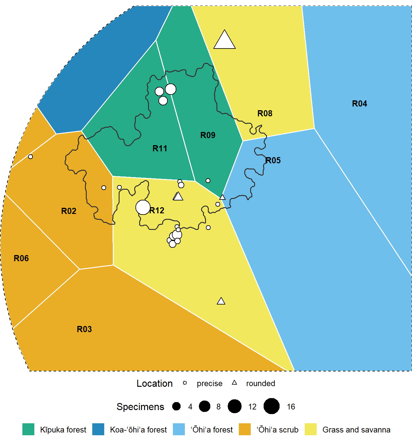
Specimens over the vegetation tiles. Circles are specimens located on the ground; triangles carry rounded coordinates. Larger symbols mean more specimens at the same coordinate. The solid grey line is the kīpuka outline from Chapter 3; the dashed line is the edge of the counting frame. Labels mark the point at the center of each tile.

6.3 Counting inside the tiles

Counting is one line. The rest is giving the counts a fair comparison. A tile with twice the area would be expected to hold twice the specimens if collecting were even. So each count is set beside the number expected from the tile’s share of the frame, and the ratio of the two says whether the tile was collected more or less than its size would suggest.

## count the specimens in each tile
count_tiles <- function(tiles, points) {
  counted <- mutate(tiles,
                    specimens = lengths(st_intersects(geometry, points)),
                    area_ha   = as.numeric(st_area(geometry)) / 10000)
  counted <- st_drop_geometry(counted)
  ## expected count if specimens were spread evenly by area
  counted <- mutate(counted,
                    expected = sum(specimens) * (area_ha / sum(area_ha)),
                    ratio    = round(specimens / expected, 1),
                    expected = round(expected, 1),
                    area_ha  = round(area_ha, 1))
  counted
}

## all specimens
tile_counts <- count_tiles(frame_tiles, frame_specimens)

## show the tiles, most collected first
tile_counts |>
  select(releve, vegetation, area_ha, specimens, expected, ratio) |>
  arrange(desc(ratio)) |>
  gt() |>
  cols_label(releve     = "Tile",
             vegetation = "Vegetation",
             area_ha    = "Area in frame (ha)",
             specimens  = "Specimens",
             expected   = "Expected by area",
             ratio      = "Ratio")

Tile	Vegetation	Area in frame (ha)	Specimens	Expected by area	Ratio
R12	Grass and savanna	88.9	47	10.9	4.3
R08	Grass and savanna	60.4	17	7.4	2.3
R11	Kīpuka forest	44.8	10	5.5	1.8
R09	Kīpuka forest	44.0	10	5.4	1.8
R02	ʻŌhiʻa scrub	51.0	2	6.3	0.3
R05	ʻŌhiʻa forest	159.2	1	19.6	0.1
R07	ʻŌhiʻa scrub	5.3	0	0.7	0.0
R10	Koa-ʻōhiʻa forest	38.3	0	4.7	0.0
R03	ʻŌhiʻa scrub	87.5	0	10.7	0.0
R06	ʻŌhiʻa scrub	28.0	0	3.4	0.0
R04	ʻŌhiʻa forest	101.2	0	12.4	0.0

6.4 The pile-up problem

Look again at the map. Some of the largest symbols are triangles: many specimens sharing one rounded coordinate. Those specimens weren’t collected at that spot. The coordinate is where someone later put a pin for “Kīpuka Puaulu,” or for a round number near it. Wherever that pin falls, its tile collects all of them.

That’s a problem with the data, not the tiles, and it’s the same friction as the one in Chapter 1. Before GPS, a botanist deep in the forest wrote down the locality, not a coordinate, and the coordinate was added later, as well as anyone could. The fair test is to count again using only the specimens located on the ground.

## only the specimens located on the ground
precise_specimens <- filter(frame_specimens, georeference == "precise")
precise_counts    <- count_tiles(frame_tiles, precise_specimens)

## compare the two counts, tile by tile
compare_counts <- left_join(
  select(tile_counts, releve, vegetation, all_specimens = specimens, all_ratio = ratio),
  select(precise_counts, releve, precise_specimens = specimens, precise_ratio = ratio),
  by = "releve")

## show it
compare_counts |>
  arrange(releve) |>
  gt() |>
  cols_label(releve            = "Tile",
             vegetation        = "Vegetation",
             all_specimens     = "All specimens",
             all_ratio         = "Ratio, all",
             precise_specimens = "Located on the ground",
             precise_ratio     = "Ratio, located")

Tile	Vegetation	All specimens	Ratio, all	Located on the ground	Ratio, located
R02	ʻŌhiʻa scrub	2	0.3	2	0.4
R03	ʻŌhiʻa scrub	0	0.0	0	0.0
R04	ʻŌhiʻa forest	0	0.0	0	0.0
R05	ʻŌhiʻa forest	1	0.1	0	0.0
R06	ʻŌhiʻa scrub	0	0.0	0	0.0
R07	ʻŌhiʻa scrub	0	0.0	0	0.0
R08	Grass and savanna	17	2.3	0	0.0
R09	Kīpuka forest	10	1.8	10	2.6
R10	Koa-ʻōhiʻa forest	0	0.0	0	0.0
R11	Kīpuka forest	10	1.8	10	2.6
R12	Grass and savanna	47	4.3	40	5.1

Of the 87 specimens in the frame, 25 carry rounded coordinates. Taking them out changes the picture tile by tile. Tile R08 goes from 17 specimens to 0: every specimen it held came from rounded coordinates. The rule it teaches is simple. A point can only be counted in a tile if its location error is small compared with the tile. These tiles are several hundred meters across. A coordinate that could be a kilometer off can’t be placed in one of them, however confidently the number is printed.

6.5 Counting by vegetation type

Tiles of the same vegetation type can be merged, as in Chapter 4, and counted as one container. Now the question becomes: which kinds of vegetation have botanists collected in, and which have they passed by?

## merge the tiles in the frame by vegetation type
type_tiles <- summarise(group_by(frame_tiles, vegetation))

## counts by type, for all specimens and for those located on the ground
type_all     <- mutate(count_tiles(type_tiles, frame_specimens), which = "All specimens")
type_precise <- mutate(count_tiles(type_tiles, precise_specimens), which = "Located on the ground")
type_counts  <- bind_rows(type_all, type_precise)

## show the table
type_counts |>
  select(which, vegetation, area_ha, specimens, expected, ratio) |>
  gt(groupname_col = "which") |>
  cols_label(vegetation = "Vegetation",
             area_ha    = "Area in frame (ha)",
             specimens  = "Specimens",
             expected   = "Expected by area",
             ratio      = "Ratio")

Vegetation	Area in frame (ha)	Specimens	Expected by area	Ratio
All specimens
Grass and savanna	149.3	64	18.3	3.5
Koa-ʻōhiʻa forest	38.3	0	4.7	0.0
Kīpuka forest	88.8	20	10.9	1.8
ʻŌhiʻa forest	260.5	1	32.0	0.0
ʻŌhiʻa scrub	171.7	2	21.1	0.1
Located on the ground
Grass and savanna	149.3	40	13.1	3.1
Koa-ʻōhiʻa forest	38.3	0	3.4	0.0
Kīpuka forest	88.8	20	7.8	2.6
ʻŌhiʻa forest	260.5	0	22.8	0.0
ʻŌhiʻa scrub	171.7	2	15.0	0.1

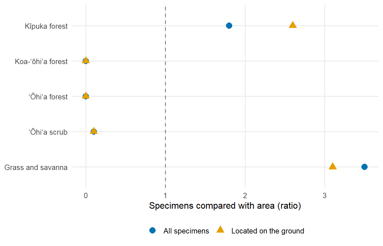
Specimens per vegetation type, compared with what area alone would predict. A ratio above 1 means the type was collected more than its area suggests. Blue: all specimens. Orange: only those located on the ground.

## draw the ratios, one row per vegetation type
ggplot(type_counts, aes(x = ratio, y = factor(vegetation, levels = rev(names(veg_colors))),
                        color = which, shape = which)) +
  geom_vline(xintercept = 1, color = "grey50", linetype = "dashed") +
  geom_point(size = 3.5) +
  scale_color_manual(values = c("All specimens" = "#0072B2", "Located on the ground" = "#E69F00"), name = NULL) +
  scale_shape_manual(values = c("All specimens" = 16, "Located on the ground" = 17), name = NULL) +
  labs(x = "Specimens compared with area (ratio)", y = NULL) +
  theme_minimal(base_size = 12) +
  theme(legend.position = "bottom", panel.grid.minor = element_blank())

Specimens per vegetation type, compared with what area alone would predict. A ratio above 1 means the type was collected more than its area suggests. Blue: all specimens. Orange: only those located on the ground.

The top of the list is a surprise: grass and savanna. The map explains it. Point R12 sits inside the kīpuka, in what the 1974 map shows as one of its grassy openings, so it’s labeled grass and savanna. But its tile covers the whole south end of the kīpuka, forest included, where the loop trail begins, and that’s where many of the specimens were collected. The count is right. It’s the label on the container that’s wrong. A count by vegetation type is only as good as the map of types, and a map from twelve points is coarse. That’s the problem Chapter 8 takes on.

6.6 What the counts measure

It’s worth being clear about what these counts are. They aren’t a measure of how many plants grow in each type. They’re a measure of where botanists went. A type with a high ratio drew collectors, perhaps because it’s rich in species, perhaps because a trail runs through it, perhaps because it has a name people know. A type with a low ratio was passed by. Here the ʻōhiʻa forest and scrub, which cover most of the frame, hold almost none of the specimens.

That turns the count into something practical. The types with low ratios are where the next collecting trip will add the most. That’s the idea behind The Briefing Books: use the herbarium’s own record to see where the gaps are before heading into the field. The tiles give that idea a map.

NoteUseful?

Yes, and the example is less obvious than it looks. Invasive plants or cases of a disease are the natural things to count inside tiles. Herbarium specimens show that any located record can be counted the same way, and that the count often measures the people who made the record as much as the thing recorded. Two cautions come with it: the counted points need their own frame, and their locations have to be good enough for the tiles they’re counted in.

The tiles give the counts a home. The coordinates decide whether they belong there.