7  Weighted Voronoi

Every map so far has treated its points as equals. Each point claims the ground nearest to it, and that’s all. But points aren’t always equal. A large, famous garden draws visitors from much farther away than a small one. A busy clinic serves more people than a quiet one.

A weighted Voronoi map lets each point pull with its own strength. This chapter leaves Kīpuka Puaulu for a while and goes to the Los Angeles basin, to five botanical gardens I’ve visited and photographed many times: the Los Angeles County Arboretum, Descanso Gardens, the Huntington, the South Coast Botanic Garden and the California Botanic Garden. The question is an old one for anyone who runs a garden. Where do our visitors come from?

It’s also a chance to show something that runs through this whole document. A tessellation isn’t only a way to draw a map. It’s a way to explore data, to ask “what if?” and see the answer at once.

## --- Standard packages ---

## many useful functions, including read_csv() and ggplot()
library(tidyverse)
## formatted tables
library(gt)

## --- Specialized packages ---

## spatial vector data: points, polygons
library(sf)
## spatial raster data: grids of cells
library(terra)
## labels that move apart so they don't overlap
library(ggrepel)

## --- Options and defaults ---

## suppress read_csv() column-type messages
options(readr.show_col_types = FALSE)

## one color per garden (Okabe-Ito palette)
garden_colors <- c("LA County Arboretum"        = "#009E73",
                   "Descanso Gardens"           = "#E69F00",
                   "The Huntington"             = "#0072B2",
                   "South Coast Botanic Garden" = "#F0E442",
                   "California Botanic Garden"  = "#D55E00")

7.1 Five gardens

## the five gardens
gardens <- read_csv("data/la_gardens.csv")

## show them
gardens |>
  select(garden, city, acres, pageviews_2024) |>
  gt() |>
  cols_label(garden         = "Garden",
             city           = "City",
             acres          = "Area (acres)",
             pageviews_2024 = "Wikipedia pageviews, 2024") |>
  fmt_number(columns = pageviews_2024, decimals = 0) |>
  tab_source_note(source_note = "Areas from Wikipedia; locations from OpenStreetMap; pageviews from the Wikimedia pageviews API (users only, 2024). Made by R/make_la_gardens_data.R.")

Garden	City	Area (acres)	Wikipedia pageviews, 2024
LA County Arboretum	Arcadia	127	10,623
Descanso Gardens	La Cañada Flintridge	150	9,969
The Huntington	San Marino	120	80,352
South Coast Botanic Garden	Palos Verdes Peninsula	87	11,999
California Botanic Garden	Claremont	86	2,472
Areas from Wikipedia; locations from OpenStreetMap; pageviews from the Wikimedia pageviews API (users only, 2024). Made by R/make_la_gardens_data.R.

Two more files set the stage. One is the frame: the land of the basin, from the coast to the foot of the mountains and out to Claremont. The ocean is left out, following Chapter 3; nobody drives to a garden from the sea. The other is the 2020 census, as one point per census tract with its population.

## the land frame, in UTM zone 11N (meters)
land <- st_read("data/la_land_frame.geojson", quiet = TRUE)
land <- st_transform(land, 32611)

## census tracts: one point each, with its 2020 population
tracts       <- read_csv("data/la_tracts_2020.csv")
tract_points <- st_as_sf(tracts, coords = c("longitude", "latitude"), crs = 4326)
tract_points <- st_transform(tract_points, 32611)

## the gardens as points
garden_points <- st_as_sf(gardens, coords = c("longitude", "latitude"), crs = 4326)
garden_points <- st_transform(garden_points, 32611)

## short names for the map labels
garden_points$short <- c("Arboretum", "Descanso", "Huntington", "South Coast", "Cal Botanic")

The frame covers about 9,521 square kilometers of land and holds 3,207 census tracts, home to 13,769,096 people.

7.2 One rule, three weights

A weighted Voronoi map needs only a small change to the rule. Instead of asking which garden is nearest, it asks which garden is nearest after dividing each distance by that garden’s weight. A garden with twice the weight seems half as far away. Give every garden a weight of 1 and the rule is the ordinary Voronoi map again.

The code below turns that rule into a function. It covers the frame with cells 500 meters across and gives each cell to the garden that wins it. The same function assigns each census tract, so the people can be counted too.

## the garden coordinates, as a two-column matrix
garden_xy <- st_coordinates(garden_points)

## for a set of locations, return the winning garden under a set of weights
winning_garden <- function(xy, weights) {
  ## weighted distance from every location to every garden
  weighted <- sapply(seq_len(nrow(garden_xy)), function(i) {
    distance <- sqrt(((xy[, 1] - garden_xy[i, 1])^2) + ((xy[, 2] - garden_xy[i, 2])^2))
    distance / weights[i]
  })
  ## the garden with the smallest weighted distance wins
  gardens$garden[max.col(-weighted)]
}

## a grid of 500 m cells covering the land
grid       <- rast(ext(vect(land)), resolution = 500, crs = "EPSG:32611")
grid       <- rasterize(vect(land), grid)
land_cells <- which(!is.na(values(grid)))
cell_xy    <- xyFromCell(grid, land_cells)

## turn a set of winners into a map of service areas
service_map <- function(weights) {
  winners <- winning_garden(cell_xy, weights)
  areas   <- grid
  values(areas)[land_cells] <- match(winners, gardens$garden)
  areas   <- st_as_sf(as.polygons(areas))
  names(areas)[1] <- "id"
  mutate(areas, garden = gardens$garden[id])
}

## draw one service-area map
draw_service <- function(areas, title) {
  ggplot() +
    geom_sf(data = areas, aes(fill = garden), color = "white", linewidth = 0.3) +
    geom_sf(data = land, fill = NA, color = "grey40", linewidth = 0.3) +
    geom_sf(data = garden_points, shape = 21, fill = "white", color = "black", size = 2.6) +
    geom_label_repel(data = garden_points, aes(label = short, geometry = geometry),
                     stat = "sf_coordinates", size = 3.4, min.segment.length = 0,
                     box.padding = 0.6, seed = 7) +
    scale_fill_manual(values = garden_colors, breaks = names(garden_colors), name = NULL, drop = FALSE) +
    coord_sf(datum = NA, expand = FALSE) +
    labs(x = NULL, y = NULL) +
    labs(title = title) +
    theme_void(base_size = 12) +
    theme(legend.position = "bottom", plot.title = element_text(face = "bold")) +
    guides(fill = guide_legend(nrow = 2))
}

## count the people each garden wins
people_won <- function(weights) {
  winners <- winning_garden(st_coordinates(tract_points), weights)
  won     <- tapply(tracts$population, factor(winners, levels = gardens$garden), sum)
  as.numeric(replace(won, is.na(won), 0))
}

7.3 The nearest garden

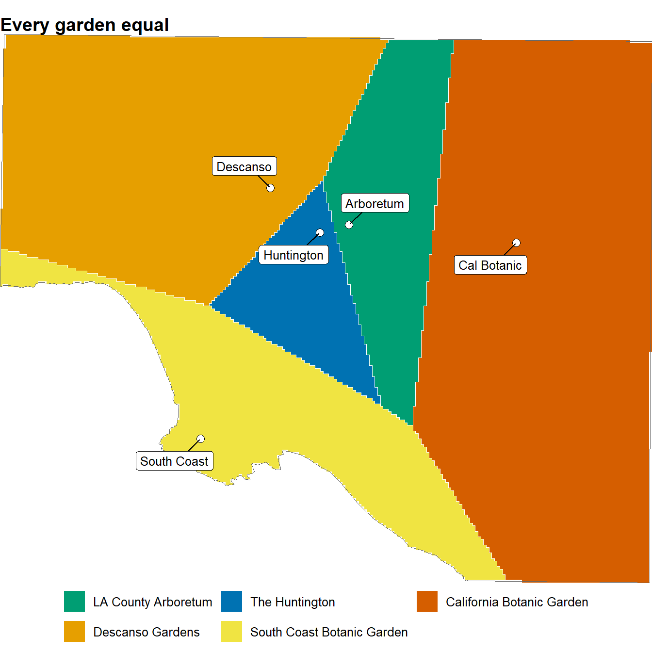
First, every garden is equal. Each one serves whoever is closest.

## all weights equal
equal_weights <- rep(1, nrow(gardens))
draw_service(service_map(equal_weights), "Every garden equal")

Service areas when every garden has the same weight: each place goes to its nearest garden.

Three of the gardens sit close together near Pasadena, so they split the middle of the basin into slices. The Huntington, in the middle of the three, gets the smallest. South Coast, alone on the Palos Verdes Peninsula, gets the whole coastal plain. The California Botanic Garden, out in Claremont, gets everything to the east.

7.4 Weighted by size

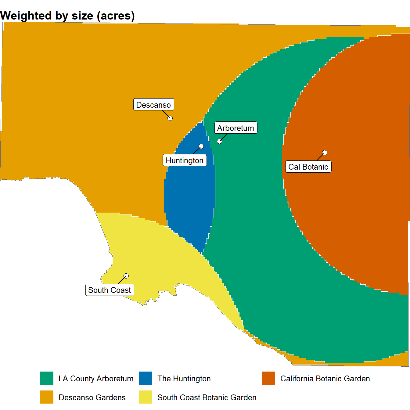
Now let the gardens pull in proportion to their size. Descanso, at 150 acres, pulls a little harder than the Huntington at 120, and much harder than the two gardens under 90 acres.

## weights equal to garden area
size_weights <- gardens$acres
draw_service(service_map(size_weights), "Weighted by size (acres)")

Service areas weighted by garden size. The edges bend into curves, and the larger gardens reach farther.

The straight edges are gone. With weights, the boundary between two gardens becomes a curve, and around a weaker garden it closes into a circle. The California Botanic Garden, the smallest, now sits inside a disk. The Huntington, squeezed between two larger neighbors, becomes a narrow lens.

Then look at the bottom edge of the map. Descanso turns up again along the coast, on the far side of the Arboretum. That isn’t a mistake. Under this rule the strongest point always wins if you go far enough, in any direction, even past its rivals. It’s the kind of result nobody would draw by hand, and the kind that makes you stop and ask whether the rule fits the way people choose.

Nothing about the gardens moved. Only the rule changed, and the map redrew itself in a second.

7.5 Weighted by public interest

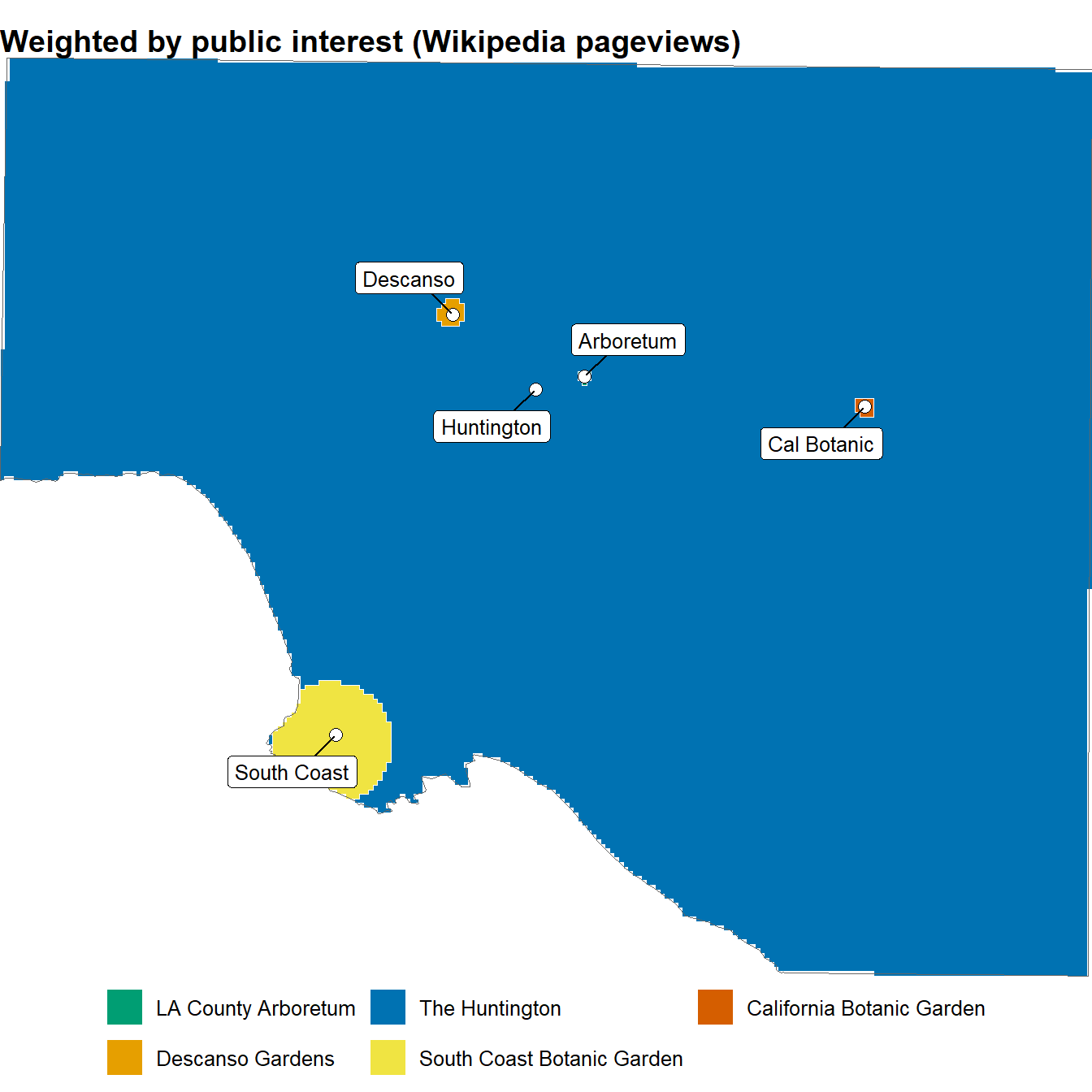
Size is one kind of pull. Fame is another. There’s no consistent record of attendance for all five gardens, but there is a consistent record of something close to fame: how often people look each garden up. The last column of the table above counts the views of each garden’s Wikipedia article in 2024.

## weights equal to 2024 pageviews
interest_weights <- gardens$pageviews_2024
draw_service(service_map(interest_weights), "Weighted by public interest (Wikipedia pageviews)")

Service areas weighted by Wikipedia pageviews. One garden takes nearly everything.

That’s a surprise, and a useful one. The Huntington’s article draws about 7 times as many views as the next garden’s, and with that weight it takes almost the whole basin. Descanso, the largest garden, and the California Botanic Garden shrink to specks around their own gates. The Arboretum, less than six kilometers from the Huntington, all but vanishes. Only South Coast, far off on its peninsula, keeps a real patch.

Part of the reason is that the Huntington’s article covers a library and an art museum as well as the gardens. Pageviews measure curiosity, not visits. But the map makes the point sharply. A weight is a theory about why people choose, and the map shows what the theory implies. A theory that gives one garden 7 times the pull of the others says that garden serves everyone, and the picture makes that claim impossible to miss.

7.6 Who lives in each service area?

The service areas are also containers, as in Chapter 6. Counting the census tracts inside each one gives the number of people for whom that garden is the choice under each rule.

## people won by each garden, under each rule
people_table <- tibble(garden    = gardens$garden,
                       equal     = people_won(equal_weights),
                       by_size   = people_won(size_weights),
                       by_interest = people_won(interest_weights))

## show it, in millions
people_table |>
  gt() |>
  cols_label(garden      = "Garden",
             equal       = "Every garden equal",
             by_size     = "Weighted by size",
             by_interest = "Weighted by interest") |>
  fmt_number(columns = c(equal, by_size, by_interest), scale_by = 1e-6, decimals = 2, pattern = "{x} M") |>
  tab_header(title = "People living in each garden's service area")

People living in each garden's service area
Garden	Every garden equal	Weighted by size	Weighted by interest
LA County Arboretum	1.11 M	4.07 M	0.01 M
Descanso Gardens	3.33 M	4.72 M	0.00 M
The Huntington	2.10 M	1.54 M	13.51 M
South Coast Botanic Garden	4.07 M	1.81 M	0.25 M
California Botanic Garden	3.16 M	1.63 M	0.01 M

The same five points and the same 13.8 million people give three very different answers. Under equal weights, South Coast serves the most people, because it has the coastal plain to itself. Weighted by size, Descanso and the Arboretum lead. Weighted by interest, the Huntington serves nearly everyone.

7.7 A check against attendance

Two of the gardens publish their attendance. The Los Angeles County Arboretum reported 572,964 visitors for its 2022-23 year. The Huntington reported 1,014,000 for 2022, a count that covers the library and art museum as well as the gardens. Set beside the people in each garden’s service area under equal weights, they give a rough rate of visits per resident.

## published attendance for the two gardens that report it
attendance <- read_csv(file =
  "garden,              visitors, period
   LA County Arboretum, 572964,   July 2022 to June 2023
   The Huntington,      1014000,  2022 (whole institution)")

## visits per resident of the equal-weight service area
attendance <- left_join(attendance, select(people_table, garden, equal), by = "garden")
attendance <- mutate(attendance, visits_per_resident = round(visitors / equal, 2))

## show it
attendance |>
  gt() |>
  cols_label(garden              = "Garden",
             visitors            = "Visitors",
             period              = "Period",
             equal               = "People in service area",
             visits_per_resident = "Visits per resident") |>
  fmt_number(columns = c(visitors, equal), decimals = 0) |>
  tab_source_note(source_note = "Los Angeles Arboretum Foundation, 2022-2023 Annual Report; Wikipedia, Huntington Library.")

Garden	Visitors	Period	People in service area	Visits per resident
LA County Arboretum	572,964	July 2022 to June 2023	1,107,462	0.52
The Huntington	1,014,000	2022 (whole institution)	2,098,389	0.48
Los Angeles Arboretum Foundation, 2022-2023 Annual Report; Wikipedia, Huntington Library.

The two rates are close. That’s only two gardens, and visitors come from far outside any service area, so it proves nothing. But it shows the kind of question the tiles make easy to ask.

7.8 What the weights mean

Weights turn a Voronoi map from a statement about distance into a statement about attraction. Size, fame, capacity and attendance are all candidates, and each one draws a different map. None of them is the right one. They’re different theories, and the map lets you see each theory’s consequences before you commit to it.

Distance itself can change too. People in Los Angeles don’t travel in straight lines. They follow the freeways, and a garden twenty kilometers away along a freeway can be closer in time than one ten kilometers away across town. Replacing straight-line distance with travel time is the same move Chapter 8 makes at Kīpuka Puaulu, where the distance that matters depends on the canopy, not the map.

NoteUseful?

Yes, and especially for exploration. A weighted map is quick to make and quick to change. It turns “what if attendance depends on size?” or “what if it depends on fame?” into a picture in seconds, and it counts the people each answer implies. The weights themselves need care: a weight is an assumption, and the map will follow it wherever it leads.

Unweighted tiles ask which garden is nearest. Weighted tiles ask which garden pulls hardest.