5  Reading the Cells

A tile map is more than a picture. Every tile is a polygon with a size and a shape, and every tile has neighbors. Those numbers come free with the map, and they say a lot, mostly about the sampling that made it.

This chapter measures the tiles three ways. First, one tile at a time. Then the pattern across all of them. Then the boundaries between vegetation types, and how far each one could be wrong.

## --- Standard packages ---

## many useful functions, including read_csv() and ggplot()
library(tidyverse)
## formatted tables
library(gt)

## --- Specialized packages ---

## spatial data: points, polygons, and the Voronoi function
library(sf)
## stacking several maps into one figure
library(patchwork)

## --- Options and defaults ---

## suppress read_csv() column-type messages
options(readr.show_col_types = FALSE)

## the vegetation colors used throughout the document (Okabe-Ito palette)
veg_colors <- c("Kīpuka forest"     = "#009E73",
                "Koa-ʻōhiʻa forest" = "#0072B2",
                "ʻŌhiʻa forest"     = "#56B4E9",
                "ʻŌhiʻa scrub"      = "#E69F00",
                "Grass and savanna" = "#F0E442")

## the twelve sample points, in UTM zone 5N
releves       <- read_csv("data/kipuka_puaulu_releves.csv")
releve_points <- st_as_sf(releves, coords = c("easting", "northing"), crs = 32605)

## the study area rectangle
area_corners <- read_csv("data/kipuka_puaulu_study_area.csv")
study_box    <- st_bbox(c(xmin = area_corners$easting[1],
                          ymin = area_corners$northing[1],
                          xmax = area_corners$easting[2],
                          ymax = area_corners$northing[2]),
                        crs = st_crs(32605))
study_area   <- st_as_sfc(study_box)

## the three tile-building steps from Chapter 2, as a function
make_tiles <- function(points, frame) {
  ## build the tiles around all the points
  tiles_all <- st_voronoi(st_union(points), envelope = frame)
  ## split the result into separate polygons
  tiles <- st_collection_extract(tiles_all)
  ## trim the tiles to the frame
  tiles <- st_intersection(tiles, frame)
  ## attach each tile to the point inside it
  tiles <- st_sf(geometry = tiles)
  st_join(tiles, points)
}

## the tiles used in this chapter, in the same order as the points
releve_tiles <- make_tiles(releve_points, study_area)
releve_tiles <- releve_tiles[match(releve_points$releve, releve_tiles$releve), ]

5.1 One tile at a time

My notes for this project listed six things worth measuring for each tile: its area, its border length, the nearest and the farthest distance from its point to its border, how many neighbors it has, and how much of its border it shares with those neighbors. All six take only a few lines.

## area and border length
tile_area_ha  <- as.numeric(st_area(releve_tiles)) / 10000
tile_border_m <- as.numeric(st_length(st_boundary(releve_tiles)))

## nearest distance from each point to its own tile's border
near_m <- as.numeric(st_distance(releve_points, st_boundary(releve_tiles), by_element = TRUE))

## farthest distance from each point to a corner of its own tile
far_m <- sapply(seq_len(nrow(releve_tiles)), function(i) {
  corners <- st_cast(st_boundary(releve_tiles[i, ]), "POINT")
  max(as.numeric(st_distance(releve_points[i, ], corners)))
})

## neighbors: tiles that share a stretch of border, not just a corner
shared <- st_relate(releve_tiles, releve_tiles, pattern = "F***1****")
n_neighbors <- lengths(shared)

## border shared with neighbors, as a share of the whole border
frame_edge   <- st_boundary(study_area)
on_frame_m   <- sapply(seq_len(nrow(releve_tiles)), function(i)
  sum(as.numeric(st_length(st_intersection(st_boundary(releve_tiles[i, ]), frame_edge)))))
shared_pct   <- round(100 * ((tile_border_m - on_frame_m) / tile_border_m))

## put them together
tile_stats <- tibble(point       = releve_tiles$releve,
                     vegetation  = releve_tiles$vegetation,
                     area_ha     = round(tile_area_ha, 1),
                     border_m    = round(tile_border_m),
                     nearest_m   = round(near_m),
                     farthest_m  = round(far_m),
                     neighbors   = n_neighbors,
                     shared_pct  = shared_pct)

## show them
tile_stats |>
  gt() |>
  cols_label(point      = "Point",
             vegetation = "Vegetation",
             area_ha    = "Area (ha)",
             border_m   = "Border (m)",
             nearest_m  = "Nearest border (m)",
             farthest_m = "Farthest corner (m)",
             neighbors  = "Neighbors",
             shared_pct = "Border shared (%)")

Point	Vegetation	Area (ha)	Border (m)	Nearest border (m)	Farthest corner (m)	Neighbors	Border shared (%)
R01	Koa-ʻōhiʻa forest	23.1	1956	147	434	2	51
R02	ʻŌhiʻa scrub	51.8	2881	239	576	6	100
R03	ʻŌhiʻa scrub	94.2	5080	302	1478	3	55
R04	ʻŌhiʻa forest	101.2	4854	339	1290	2	44
R05	ʻŌhiʻa forest	159.2	5062	170	1798	4	70
R06	ʻŌhiʻa scrub	63.2	3509	239	909	3	62
R07	ʻŌhiʻa scrub	39.0	2614	168	645	4	64
R08	Grass and savanna	60.4	3210	170	925	3	76
R09	Kīpuka forest	44.0	3136	177	951	5	96
R10	Koa-ʻōhiʻa forest	62.0	3227	147	951	5	72
R11	Kīpuka forest	44.8	2857	177	768	4	100
R12	Grass and savanna	88.9	4279	220	1510	5	99

Two of the columns deserve a closer look.

Nearest border. For a tile with neighbors all round, the nearest border is exactly halfway to the nearest other point. Double it and you have the distance to that point. So this column is really a record of sampling spacing, read straight off the map.

Farthest corner. This is the farthest place that the point’s category is being stretched to cover. A sample whose tile reaches a kilometer away is making a much bigger claim than one whose tile reaches 200 meters.

Arnold and Milne (1984) used the same idea as a check on their field crews. The Greek survey was meant to sample every 50 to 200 meters, and the distances to each point’s nearest and farthest neighbors showed whether it had. The map audits the sampling that made it.

The last column comes from Chapter 3. A tile that shares only part of its border with other tiles is an edge tile, and part of its shape comes from the frame.

5.2 The pattern across the tiles

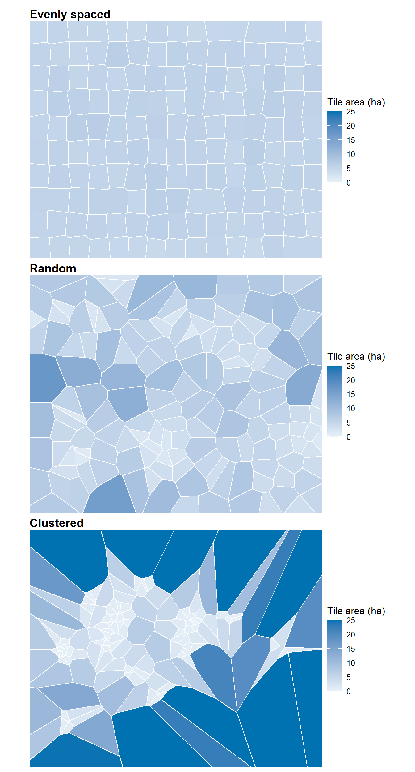
The tiles together say something about how the points were placed. If the points are spread evenly, the tiles are all about the same size. If the points were placed at random, the sizes vary. If the points are clustered, some tiles are small and crowded and others are large, sitting in the gaps between the clusters.

A single number captures this: the coefficient of variation of tile area, the standard deviation divided by the mean. The code below makes three sets of 150 points in the Kīpuka Puaulu rectangle, one evenly spaced, one random and one clustered, and measures each. Only interior tiles count, so the frame doesn’t distort the result.

## the same random numbers every time the chapter is run
set.seed(1984)

## rectangle limits, for placing points
x_min <- area_corners$easting[1];  x_max <- area_corners$easting[2]
y_min <- area_corners$northing[1]; y_max <- area_corners$northing[2]

## pattern 1: an even grid of 15 by 10 points, nudged slightly
grid_x <- seq(x_min + 100, x_max - 100, length.out = 15)
grid_y <- seq(y_min + 100, y_max - 100, length.out = 10)
even   <- expand_grid(easting = grid_x, northing = grid_y)
even   <- mutate(even, easting  = easting  + runif(n(), -25, 25),
                       northing = northing + runif(n(), -25, 25))

## pattern 2: 150 points placed at random
random <- tibble(easting  = runif(150, x_min, x_max),
                 northing = runif(150, y_min, y_max))

## pattern 3: 15 cluster centers with 10 points around each
centers   <- tibble(cx = runif(15, x_min + 300, x_max - 300),
                    cy = runif(15, y_min + 300, y_max - 300))
clustered <- tibble(easting  = rep(centers$cx, each = 10) + rnorm(150, 0, 90),
                    northing = rep(centers$cy, each = 10) + rnorm(150, 0, 90))

## keep every point inside the rectangle
clustered <- filter(clustered, between(easting, x_min, x_max), between(northing, y_min, y_max))

## build tiles for one pattern and flag the interior tiles
pattern_tiles <- function(pts, label) {
  pts   <- st_as_sf(pts, coords = c("easting", "northing"), crs = 32605)
  pts   <- mutate(pts, id = row_number())
  tiles <- make_tiles(pts, study_area)
  tiles <- mutate(tiles,
                  area_ha  = as.numeric(st_area(geometry)) / 10000,
                  interior = lengths(st_intersects(geometry, frame_edge)) == 0,
                  pattern  = label)
  tiles
}

## tiles for all three patterns
tiles_even      <- pattern_tiles(even, "Evenly spaced")
tiles_random    <- pattern_tiles(random, "Random")
tiles_clustered <- pattern_tiles(clustered, "Clustered")

## coefficient of variation of interior tile area, for each pattern
cv_of <- function(tiles) {
  a <- tiles$area_ha[tiles$interior]
  round(sd(a) / mean(a), 2)
}
pattern_summary <- tibble(pattern        = c("Evenly spaced", "Random", "Clustered"),
                          interior_tiles = c(sum(tiles_even$interior),
                                             sum(tiles_random$interior),
                                             sum(tiles_clustered$interior)),
                          cv_area        = c(cv_of(tiles_even),
                                             cv_of(tiles_random),
                                             cv_of(tiles_clustered)))

## show it
pattern_summary |>
  gt() |>
  cols_label(pattern        = "Pattern",
             interior_tiles = "Interior tiles",
             cv_area        = "Coefficient of variation of tile area")

Pattern	Interior tiles	Coefficient of variation of tile area
Evenly spaced	104	0.07
Random	113	0.46
Clustered	127	1.46

## one map for one pattern, shaded by tile area
pattern_map <- function(tiles, title) {
  ggplot() +
    geom_sf(data = tiles, aes(fill = area_ha), color = "white", linewidth = 0.4) +
    scale_fill_gradient(low = "#e8f1f8", high = "#0072B2", name = "Tile area (ha)",
                        limits = c(0, 25), oob = scales::squish) +
    coord_sf(datum = NA, expand = FALSE) +
    labs(title = title) +
    theme_void(base_size = 12) +
    theme(legend.position = "right", plot.title = element_text(face = "bold"))
}

## stack the three maps, one per row
pattern_map(tiles_even, "Evenly spaced") /
  pattern_map(tiles_random, "Random") /
  pattern_map(tiles_clustered, "Clustered")

Tiles from 150 points placed three ways. Darker tiles are larger. Even spacing gives even tiles; clustering leaves large tiles in the gaps.

## twenty more random sets of 150 points, to see how much the random value varies
random_cvs <- sapply(1:20, function(k) {
  pts <- tibble(easting  = runif(150, x_min, x_max),
                northing = runif(150, y_min, y_max))
  cv_of(pattern_tiles(pts, "Random"))
})

For points scattered at random, the coefficient of variation of tile area comes out close to 0.5. Twenty more trials in this rectangle, with 150 random points each time, gave values from 0.43 to 0.63. Well below that range means the points were spread more evenly than chance. Well above it means they’re clustered, and the largest tiles mark the gaps between clusters.

That’s useful in two ways. For samples, large tiles are gaps in the sampling, the places where a map is stretched thinnest. For plants, if the points are the stems of trees, large tiles can be real openings in the canopy, and tile area becomes the space each tree has to grow. Plant ecologists have used the tiles that way, as the area available to each plant, in studies of competition (Brown 1965; Mead 1966).

5.3 How sure is each boundary?

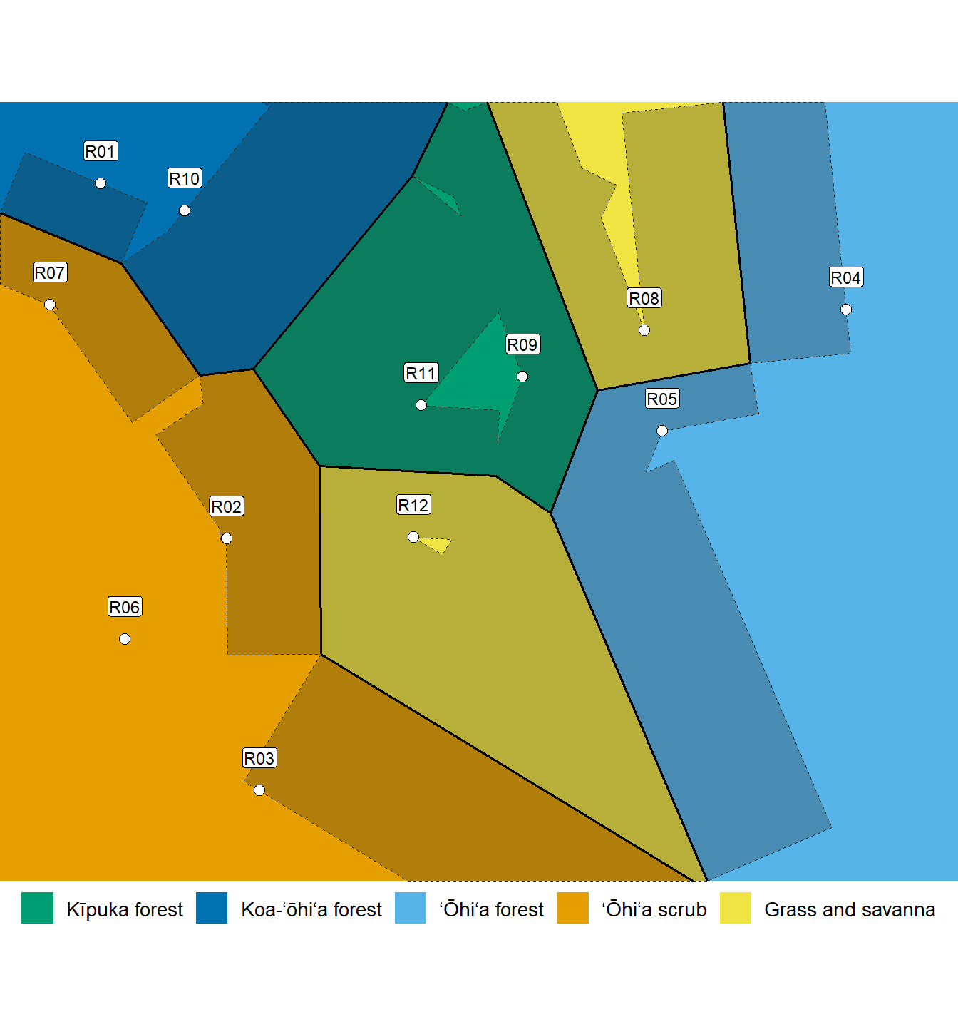
The boundary between two vegetation types on a tile map sits halfway between two samples that disagree. One sample says forest, its neighbor says scrub, and the map draws the line at the midpoint. But nothing says the real change happens there. It could be anywhere between the two samples.

So each boundary carries its own uncertainty: up to half the distance between the two samples on either side of it. That’s local. A boundary between close samples is pinned down tightly. A boundary between distant samples is not. And it can be computed for every boundary on the map.

## every pair of neighboring tiles whose vegetation differs
pairs <- which(st_relate(releve_tiles, releve_tiles, pattern = "F***1****", sparse = FALSE), arr.ind = TRUE)
pairs <- pairs[pairs[, 1] < pairs[, 2], , drop = FALSE]
differs <- releve_tiles$vegetation[pairs[, 1]] != releve_tiles$vegetation[pairs[, 2]]
pairs <- pairs[differs, , drop = FALSE]

## for each pair: the shared edge, the spacing of the two points, and a band of half that width
edges <- lapply(seq_len(nrow(pairs)), function(k) {
  i <- pairs[k, 1]; j <- pairs[k, 2]
  edge    <- st_intersection(st_geometry(releve_tiles[i, ]), st_geometry(releve_tiles[j, ]))
  spacing <- as.numeric(st_distance(releve_points[i, ], releve_points[j, ]))
  st_sf(side_a    = releve_tiles$vegetation[i],
        side_b    = releve_tiles$vegetation[j],
        spacing_m = round(spacing),
        plus_minus_m = round(spacing / 2),
        geometry  = st_collection_extract(edge, "LINESTRING") |> st_union())
})
edges <- do.call(rbind, edges)

## the band around each boundary (square ends), trimmed to the study area
bands <- st_buffer(edges, edges$plus_minus_m, endCapStyle = "FLAT")
bands <- st_intersection(bands, study_area)

## all the bands together, as one shape
band_zone <- st_union(bands)

## show the boundaries, closest samples first
edges |>
  st_drop_geometry() |>
  arrange(spacing_m) |>
  gt() |>
  cols_label(side_a       = "One side",
             side_b       = "Other side",
             spacing_m    = "Samples apart (m)",
             plus_minus_m = "Boundary could move (± m)")

One side	Other side	Samples apart (m)	Boundary could move (± m)
ʻŌhiʻa forest	Grass and savanna	340	170
Grass and savanna	Kīpuka forest	434	217
Koa-ʻōhiʻa forest	ʻŌhiʻa scrub	439	220
Kīpuka forest	Grass and savanna	441	220
ʻŌhiʻa forest	Kīpuka forest	499	249
ʻŌhiʻa scrub	Koa-ʻōhiʻa forest	549	275
ʻŌhiʻa scrub	Grass and savanna	625	313
Kīpuka forest	Grass and savanna	648	324
ʻŌhiʻa forest	Grass and savanna	679	339
ʻŌhiʻa scrub	Kīpuka forest	788	394
ʻŌhiʻa forest	Grass and savanna	903	451
ʻŌhiʻa scrub	Grass and savanna	990	495
Koa-ʻōhiʻa forest	Kīpuka forest	1023	512
ʻŌhiʻa scrub	Koa-ʻōhiʻa forest	1104	552
Kīpuka forest	Koa-ʻōhiʻa forest	1259	629

## merge tiles of the same type, as in Chapter 4
patches <- summarise(group_by(releve_tiles, vegetation))

## draw the patches, the uncertainty bands and the boundaries
ggplot() +
  geom_sf(data = patches, aes(fill = vegetation), color = NA) +
  geom_sf(data = band_zone, fill = "grey15", alpha = 0.28, color = "grey15", linewidth = 0.3, linetype = "dashed") +
  geom_sf(data = edges, color = "black", linewidth = 0.7) +
  geom_sf(data = releve_points, shape = 21, fill = "white", color = "black", size = 2.4) +
  geom_sf_label(data = releve_points, aes(label = releve), nudge_y = 110, size = 3,
                label.padding = unit(0.1, "lines"), fill = "white") +
  scale_fill_manual(values = veg_colors, breaks = names(veg_colors), name = NULL) +
  coord_sf(datum = NA, expand = FALSE) +
  theme_void(base_size = 13) +
  theme(legend.position = "bottom")

Each boundary between vegetation types (black), inside a shaded zone showing how far it could move: half the distance between the two samples that set it.

With only twelve samples, the bands are wide. About 59 percent of the study area lies within reach of a boundary that could plausibly be somewhere else. That’s an honest picture of what twelve points can say. More samples narrow the bands. So does outside information about where the edges really are, which is where Chapter 8 goes.

NoteUseful?

Yes, and it comes free. The tiles report on the sampling behind the map: its spacing, its gaps and its clustering. The boundary bands say how far each line could be wrong. A hand-drawn map can’t do either, because nothing in it records the evidence behind each line.

The tiles map the vegetation. Their sizes map the sampling.

Arnold, D. B., and W. J. Milne. 1984. “The Use of Voronoi Tessellations in Processing Soil Survey Results.” IEEE Computer Graphics and Applications 4 (3): 22–28.

Brown, G. S. 1965. “Point Density in Stems Per Acre.” Forest Research Notes 38. New Zealand Forest Service, Forest Research Institute.

Mead, R. 1966. “A Relationship Between Individual Plant-Spacing and Yield.” Annals of Botany 30 (2): 301–9.