3  The two-way table

The ragged list was the right shape for getting the data in, because it matched how you collected it. It is the wrong shape for finding pattern. To see which items go together, and which places resemble each other, we need to lay the same information out as a grid: the items down the side, the places across the top, and in each cell a mark for whether that item was at that place. This grid is the two-way table, and almost everything from here on is built on it.

## data wrangling, tables, and dendrograms
library(tidyverse)
library(gt)
library(ggdendro)

## the listsr package: the list -> tree + assessment-line toolkit
library(listsr)

## the running example, read in again
data_source <- "Source: a fish-market toy (a designed example)."
data_rows <-
"Stall1, Mussels, Crab, Lobster, Shrimp, Oysters, Clams
 Stall2, Clams, Mussels, Shrimp, Crab
 Stall3, Oysters, Crab, Lobster, Clams
 Stall4, Mackerel, Cod, Tuna, Snapper, Salmon
 Stall5, Snapper, Tuna, Salmon
 Stall6, Salmon, Mackerel, Tuna
 Stall7, Snapper, Clams, Shrimp, Tuna"
fish <- read_lists(data_rows)

3.1 From a list to a grid

One function does the reshaping. data_to_2way() takes the list we read in and turns it on its side: a row for each distinct item, a column for each stall, and in every cell a 1 if that stall sold that item or a 0 if it did not.

## reshape the list into the binary two-way table
two_way <- data_to_2way(fish)

gt(two_way) |>
  tab_source_note(data_source)

The fish market as a two-way table. A 1 marks an item sold at a stall; a 0 marks its absence.

Item	Stall1	Stall2	Stall3	Stall4	Stall5	Stall6	Stall7
Clams	1	1	1	0	0	0	1
Cod	0	0	0	1	0	0	0
Crab	1	1	1	0	0	0	0
Lobster	1	0	1	0	0	0	0
Mackerel	0	0	0	1	0	1	0
Mussels	1	1	0	0	0	0	0
Oysters	1	0	1	0	0	0	0
Salmon	0	0	0	1	1	1	0
Shrimp	1	1	0	0	0	0	1
Snapper	0	0	0	1	1	0	1
Tuna	0	0	0	1	1	1	1
Source: a fish-market toy (a designed example).

3.2 Presence and absence

The table is binary: every cell is a one or a zero, present or absent. There is nothing else in it — no prices, no quantities, no how-much — and that turns out to be a strength rather than a poverty.

It is a strength for two reasons. The first is practical: presence and absence are fast to record. You do not have to weigh the catch or count the crates; you only note that the stall had Tuna, and move on. Because each observation costs so little, you can afford to visit more stalls, and more places almost always tells you more than more detail about a few. The second reason is that the zeros are real data, not gaps. That Stall4 had no clams is as true and as informative as that it had tuna — the absences are half of what separates one kind of stall from another. A two-way table is mostly zeros, and the empty cells are doing as much work as the full ones.

For finding the large patterns we are after, presence and absence is enough.

3.3 The same table, as a picture

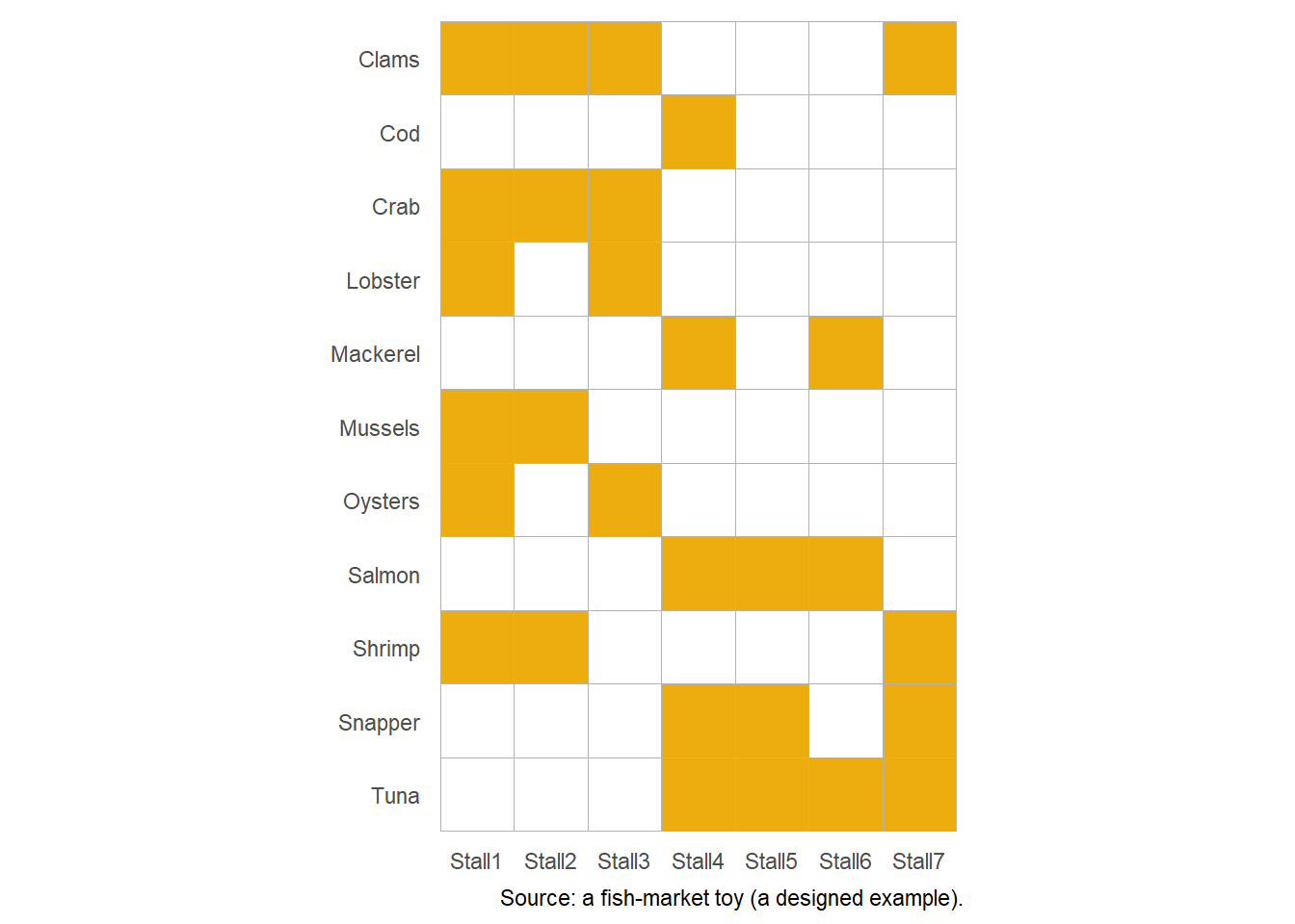
A grid of ones and zeros is precise but hard to feel. The same table drawn as a picture — a filled square for each presence, blank for each absence — is much easier to read at a glance.

two_way_plot(two_way, caption = data_source)

The two-way table as a presence/absence picture. Filled squares are presences; the white is most of the table.

Two things show up immediately. The table really is mostly empty — most of what could have been on each stall is not. And there is structure here, if you squint: a block of shellfish (Clams, Crab, Lobster, Mussels, Oysters, Shrimp) filling the first three stalls, a block of finfish (Cod, Mackerel, Salmon, Snapper, Tuna) filling the next three, and Stall7 reaching a foot into each. But the blocks are broken up and scattered, because the items are in alphabetical order and the stalls in the order we happened to type them. The pattern is present but not arranged.

That is the whole reason the two-way table matters. It does not interpret itself — you will rarely stare at one and read off an answer. What it does is hold the data in the one shape that lets the next step arrange it, sliding related items next to related items and related stalls beneath them until the scattered blocks line up and the pattern becomes plain. That arranging is the work of the next chapter, where we let the data sort itself into a tree.