2  A first look

Before reaching for anything clever, count. Two questions answer themselves from a list alone, and either one can be asked in the field, on the spot: how widespread is each thing, and how much does each place hold? Neither finds a pattern — that comes later — but both describe the data in a glance, and both catch mistakes while they are still cheap to fix.

## data wrangling, tables, and dendrograms
library(tidyverse)
library(gt)
library(ggdendro)

## the listsr package: the list -> tree + assessment-line toolkit
library(listsr)

## the running example, read in again (see "Getting the data in")
data_source <- "Source: a fish-market toy (a designed example)."
data_rows <-
"Stall1, Mussels, Crab, Lobster, Shrimp, Oysters, Clams
 Stall2, Clams, Mussels, Shrimp, Crab
 Stall3, Oysters, Crab, Lobster, Clams
 Stall4, Mackerel, Cod, Tuna, Snapper, Salmon
 Stall5, Snapper, Tuna, Salmon
 Stall6, Salmon, Mackerel, Tuna
 Stall7, Snapper, Clams, Shrimp, Tuna"
fish <- read_lists(data_rows)

2.1 How widespread is each item

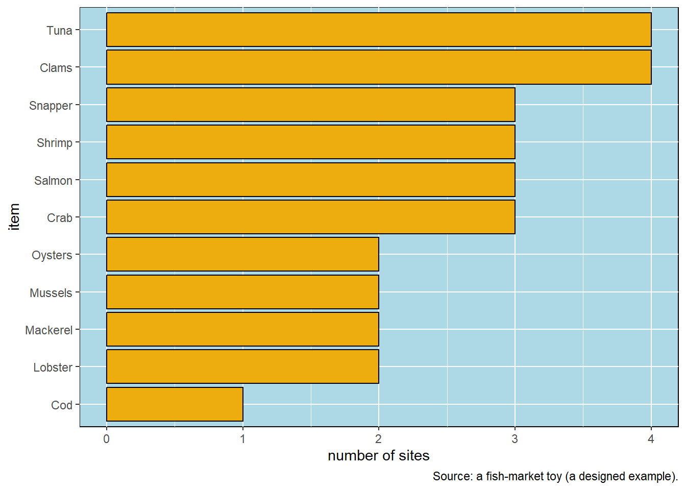
The first scan counts, for each kind of fish, the number of stalls that carried it, and sorts the result so the common things rise to the top.

item_freq_plot(fish, caption = data_source)

How many stalls carried each item, most widespread at the top.

Two items sit at the top: Clams and Tuna, each on four of the seven stalls. One sits alone at the bottom: Cod, at a single stall. The rest fall in between, on two or three stalls apiece.

It is worth pausing on what the two ends mean, because it foreshadows the whole method. An item on nearly every stall cannot tell one stall from another — if everyone sells Clams, then selling Clams says nothing about which kind of stall you are looking at. An item on a single stall is the opposite problem: it marks that one stall, but with only one occurrence it has nothing to share a pattern with. The items that distinguish groups of stalls are the ones in the middle, common enough to recur but particular enough to mean something. For now this is only an observation from a bar chart, but we will lean on it hard before the book is done.

This chart is also a quiet data check. If a fish had turned up on every stall, or if a name you did not expect appeared here, this is where you would catch it — a moment’s glance, before any of it could mislead you.

2.2 How much does each stall hold

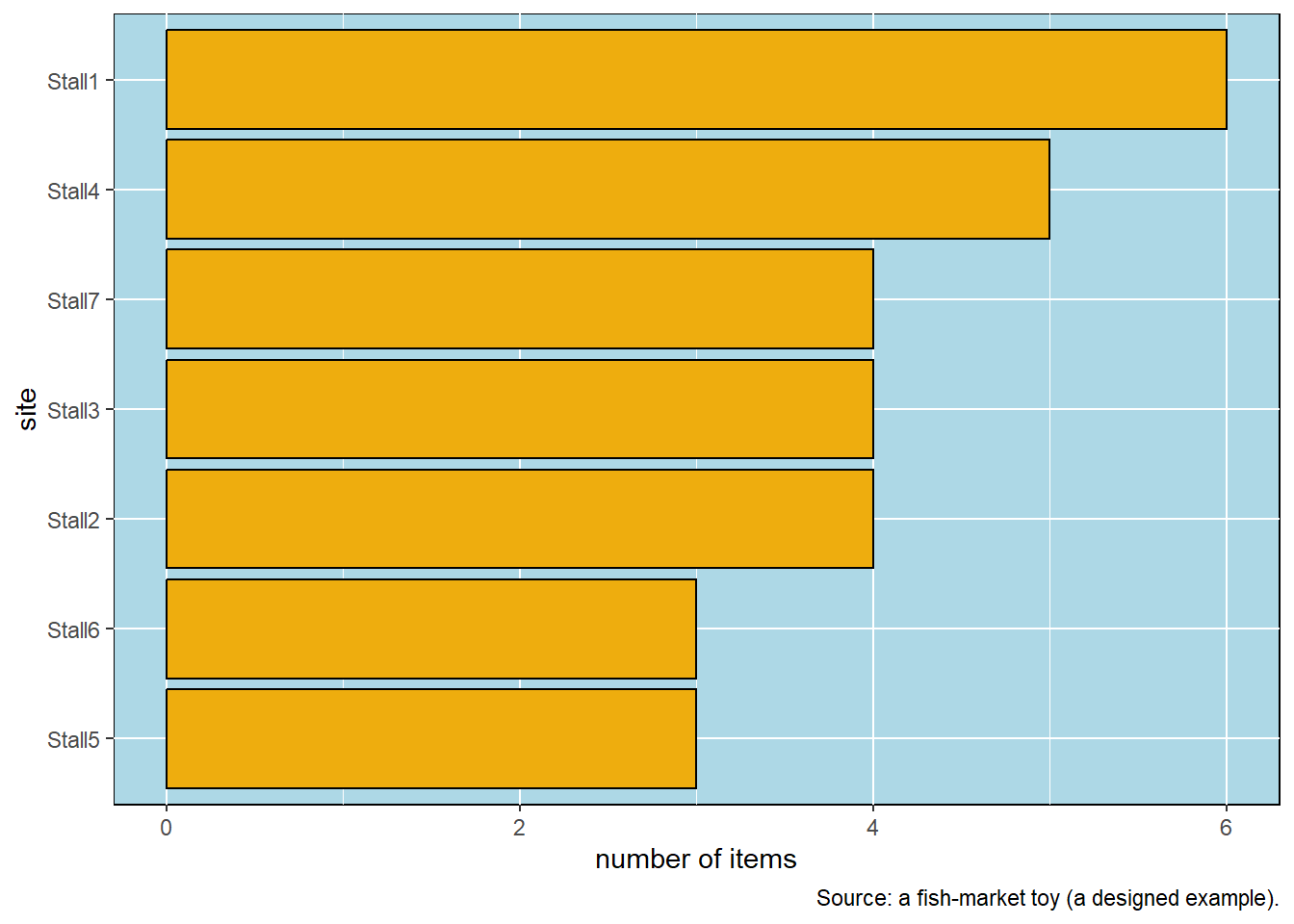
The second scan turns the same count the other way: for each stall, how many different items it carried.

site_freq_plot(fish, caption = data_source)

How many items each stall carried, largest at the top.

Stall1 is the broadest, with six kinds of fish and shellfish; Stall5 and Stall6 are the narrowest, with three. There is nothing to interpret deeply here — a stall is not better for being bigger — but the scan earns its place as a sanity check. A stall showing just one item, or one showing implausibly many, is a cue to go back to your photographs before going further.

Neither chart sorts anything or names a group. They only describe. But they take seconds, they catch errors early, and they already point at where the structure will be: the items that are everywhere or nowhere will not drive it, and the stalls differ enough in what they hold that there is clearly something to find. The next chapter lays the list out in the shape that lets us find it — the two-way table.