The two-way table holds the data, but it does not yet say what we want to know: which stalls resemble each other, and which items keep the same company. To get there we need a single idea — how alike are two things? — turned into a single number for every pair. Collect those numbers and you have a matrix, and that matrix, not the tree, is where the pattern actually lives. The dendrogram of the next chapter is only a way of looking at it.
Show the code
## data wrangling, tables, and dendrogramslibrary(tidyverse)library(gt)library(ggdendro)## the listsr package: the list -> tree + assessment-line toolkitlibrary(listsr)## the running example, read in againdata_source <-"Source: a fish-market toy (a designed example)."data_rows <-"Stall1, Mussels, Crab, Lobster, Shrimp, Oysters, Clams Stall2, Clams, Mussels, Shrimp, Crab Stall3, Oysters, Crab, Lobster, Clams Stall4, Mackerel, Cod, Tuna, Snapper, Salmon Stall5, Snapper, Tuna, Salmon Stall6, Salmon, Mackerel, Tuna Stall7, Snapper, Clams, Shrimp, Tuna"fish <-read_lists(data_rows)two_way <-data_to_2way(fish)
4.1 How unalike are two stalls?
Two stalls are alike to the degree they sell the same things. Put the other way round — which turns out to be the more useful way — they are dissimilar to the degree they do not. Take every item that either stall sold, and ask what fraction of those items only one of the two had. If the two stalls sold identical lists, that fraction is zero: no dissimilarity at all. If they shared nothing, it is one. Everything real falls in between.
That is the whole measure. It uses only presence and absence, it ignores the order things were listed in, and it gives back a single number between zero and one for every pair of stalls. The measure even has a name — the Jaccard dissimilarity — and it is just one of several ways to turn presence and absence into a distance. Which one to use is itself a choice, and a later chapter takes it up; for now it does the plain, sensible thing. dissimilarity() works it out for all pairs at once.
Show the code
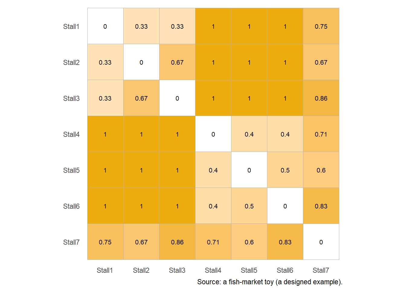
## one number per pair of stalls, shown as a matrixdissimilarity(two_way, what ="site") |>dissimilarity_plot(caption = data_source)
Stall-to-stall dissimilarity. 0 (palest) means identical lists; 1 (darkest) means nothing in common.
Read it like a small map. The diagonal is white — every stall is identical to itself. Off the diagonal, two pale blocks stand out: the first three stalls are close to one another (a third of their items differ, no more), and so are the next three. Between those two blocks runs a wall of ones: not a single shellfish stall shares anything with a single finfish stall. And the seventh stall, the mixed one, is middling to everybody — never identical to anyone, but never wholly different either, the only stall that reaches across the divide.
Everything we are looking for is already in this picture. The two groups are the two pale blocks; the gap between them is the wall of ones; the awkward case is the row that will not commit. The matrix has found the pattern.
4.2 Items, measured the same way
The identical idea turns the other way. Two items are alike to the degree they turn up at the same stalls — Tuna and Salmon, say, which travel together from stall to stall. dissimilarity(two_way, what = "item") produces the matching matrix for the eleven items, built by exactly the same rule. We will not print it here; it is larger, and we are about to meet it in a far more readable form.
Because that is the catch. The stall matrix above is seven rows of seven, and even that takes a moment to take in; the item matrix is eleven by eleven. A matrix holds the answer but hides it in a thicket of numbers, and the more sites or items you gather, the worse the thicket. What we need is a way to take this same matrix and lay it out so the eye can read it in one look — the close pairs near each other, the groups gathered, the loner set apart. That is exactly what a dendrogram does, and it is the next chapter.