The tree has done its work. From nothing but the lists — what each stall happened to sell — it proposed a grouping. But a grouping is only worth having if you can connect it to something you care about, and that something almost always lives outside the list: the owner’s name, the price, the season, where the fish was caught. Facts you keep in another column, or another file, and never fed to the analysis. Those facts are the metadata, and linking them to the groups is where the work finally pays off. Two things can happen when you bring them in, and both are useful. The metadata may agree with the groups, which is a powerful check. Or it may add a fact the lists could never have revealed.
Show the code
## data wrangling, tables, dendrogramslibrary(tidyverse)library(gt)library(ggdendro)## the listsr package: the list -> tree + assessment-line toolkitlibrary(listsr)## the running example, read in againdata_source <-"Source: a fish-market toy (a designed example)."data_rows <-"Stall1, Mussels, Crab, Lobster, Shrimp, Oysters, Clams Stall2, Clams, Mussels, Shrimp, Crab Stall3, Oysters, Crab, Lobster, Clams Stall4, Mackerel, Cod, Tuna, Snapper, Salmon Stall5, Snapper, Tuna, Salmon Stall6, Salmon, Mackerel, Tuna Stall7, Snapper, Clams, Shrimp, Tuna"fish <-read_lists(data_rows)two_way <-data_to_2way(fish)## the metadata — kept separately, never seen by the analysisstall_info <-tibble(Site =paste0("Stall", 1:7),owner =c("Santos","Reyes","Cruz","Tanaka","Yamamoto","Nakamura","Kahale"),heritage =c("Filipino","Filipino","Filipino","Japanese","Japanese","Japanese","Hawaiian"))item_info <- two_way |>transmute(Item, origin =if_else(Item =="Cod", "imported", "local"))
7.1 A second table
Here is something we know about the seven stalls that is nowhere in their sales lists: who runs each one.
The market has three communities of fishmongers. None of this touched the analysis — the tree was built from fish alone and never saw a single owner’s name. That independence is exactly what makes the next step worth taking: because the community column was withheld from the lists, it can be used to test the grouping rather than merely decorate it.
7.2 Does anything outside the data agree?
Colour the tree’s leaves by who owns each stall.
Show the code
pal_h <-c(Filipino ="#0072B2", Japanese ="#D55E00", Hawaiian ="#009E73")dissimilarity(two_way, what ="site") |>dendrogram_meta_plot(info = stall_info, by ="Site", key ="heritage",extra ="owner", palette = pal_h, caption = data_source)
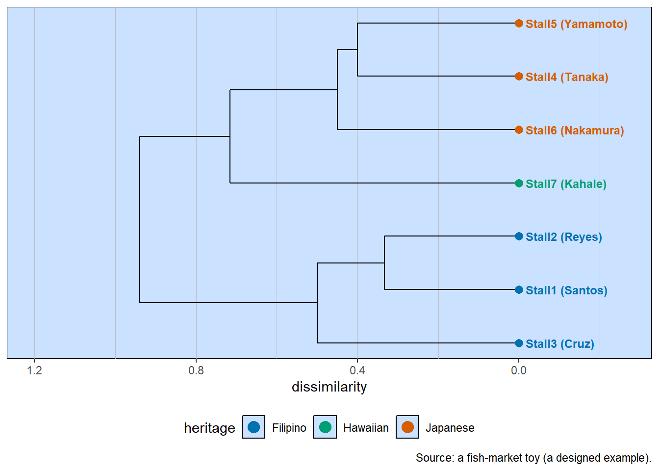
The stall tree, leaves coloured by the owner’s community — a fact the analysis never saw.
The branches and the colours tell the same story. Cut the tree into two and you separate the Filipino-owned stalls, with their shellfish, from everyone else. Cut it into three and the mixed stall steps out on its own — and now the three branches are precisely the three communities.
Show the code
g3 <-cutree(hclust(dissimilarity(two_way, what ="site"), method ="average"), k =3)tibble(Site =names(g3), tree_group =paste("group", g3)) |>left_join(stall_info, by ="Site") |>select(Site, owner, community = heritage, tree_group) |>gt() |>cols_label(Site ="stall", tree_group ="tree group (cut into 3)") |>tab_options(table.font.size =px(13))
stall
owner
community
tree group (cut into 3)
Stall1
Santos
Filipino
group 1
Stall2
Reyes
Filipino
group 1
Stall3
Cruz
Filipino
group 1
Stall4
Tanaka
Japanese
group 2
Stall5
Yamamoto
Japanese
group 2
Stall6
Nakamura
Japanese
group 2
Stall7
Kahale
Hawaiian
group 3
Stop and notice what happened. A method that knew only what was for sale recovered who was selling it. The lists never mentioned community, yet the grouping fell along it exactly. When an outside fact you withheld from the analysis lines up with the groups the analysis produced, that agreement is the cheapest and strongest validation you can get: it says the grouping is not an artifact of your distance measure or your linkage — something real, out in the world, predicts it.
Two honest qualifications keep this in proportion. The agreement is corroboration, not proof; it tells you the split is real enough that an independent fact tracks it, not that you have uncovered a law of nature. And we cut the tree by eye — two groups, or three? — the very judgement the last chapter warned against. The principled way to make that cut — letting the data’s own most variable member set how loose a group may be — is the subject of the next chapter. For now the eye and the colours agree, which is reason enough.
7.3 A fact the lists cannot see
Metadata need not agree with the groups, and the second kind is just as valuable. Most of what this market sells is caught in local waters; one item, the cod, is brought in from far colder seas. Flag the items by where they come from and look again.
Show the code
pal_o <-c(local ="#0072B2", imported ="#D55E00")dissimilarity(two_way, what ="item") |>dendrogram_meta_plot(info = item_info, by ="Item", key ="origin",palette = pal_o, caption = data_source)
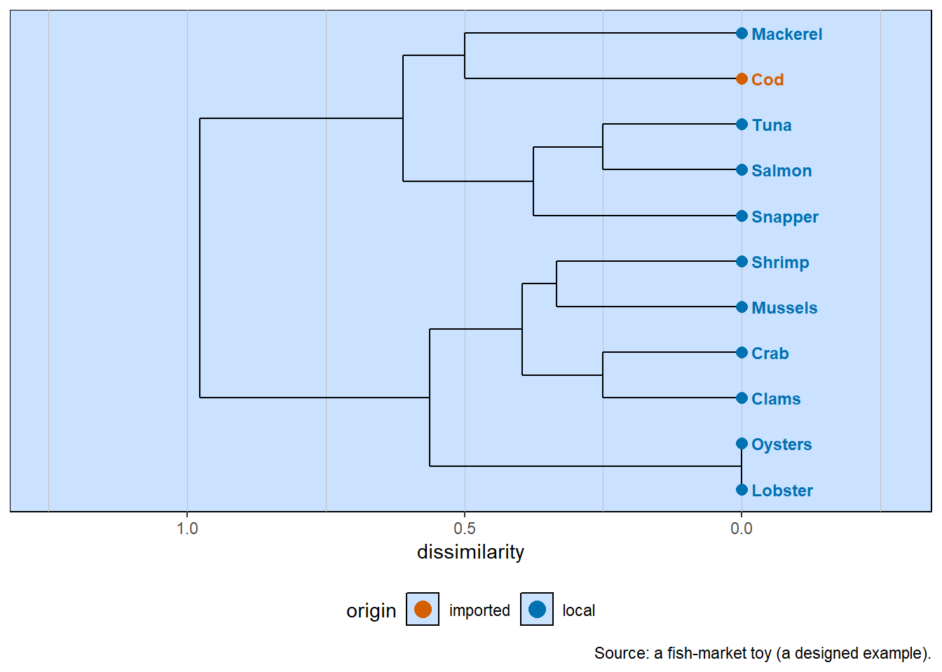
The item tree, leaves coloured by origin. The imported item does not form its own branch.
The imported cod does not break away into an “imported” branch of its own. It sits quietly inside the finfish, paired with the mackerel, because the stalls stock by kind, not by provenance — and kind is all the lists ever recorded. The origin is a true fact about the cod that no amount of clustering could recover, because it was never in the data. Here the metadata cuts across the groups instead of confirming them, and that too is information: it tells you that “where it came from” and “what sort of thing it is” are different questions, and your lists answered only one of them.
7.4 What metadata is for
A grouping earns its keep by what you can hang on it. The lists gave us reproducible groups; the metadata gives them meaning — community, provenance, price, season, anything you troubled to record alongside. And the linking disciplines you in both directions. When an outside fact agrees with the groups, your confidence rises and you have something real to explain. When an outside fact cuts across them, you are reminded that the tree knows only what you put into it, and that the question worth asking may live in a column the clustering never touched.
One loose end remains, the one the colours quietly papered over: we keep cutting the tree by eye. The next chapter replaces the eye with a rule. Letting the most variable member of a group set how loose that group may be, it draws a line across the tree that says — defensibly, and the same way every time — here is where a group begins and ends, turning a confident guess into a measurement anyone can repeat.