The matrix from the last chapter held the answer, but it held it the way a phone book holds your friend’s number: in there somewhere, surrounded by everything else. Seven stalls made a grid of forty-nine numbers; eleven items would make a hundred and twenty-one. What we need is a way to take that same matrix and lay it out so the eye can read it whole — the close pairs side by side, the groups gathered, the loner off on its own. A dendrogram does exactly that. It is not a new analysis. It is the matrix, drawn as a tree.
Show the code
## data wrangling, tables, and dendrogramslibrary(tidyverse)library(gt)library(ggdendro)## the listsr package: the list -> tree + assessment-line toolkitlibrary(listsr)## the running example, read in againdata_source <-"Source: a fish-market toy (a designed example)."data_rows <-"Stall1, Mussels, Crab, Lobster, Shrimp, Oysters, Clams Stall2, Clams, Mussels, Shrimp, Crab Stall3, Oysters, Crab, Lobster, Clams Stall4, Mackerel, Cod, Tuna, Snapper, Salmon Stall5, Snapper, Tuna, Salmon Stall6, Salmon, Mackerel, Tuna Stall7, Snapper, Clams, Shrimp, Tuna"fish <-read_lists(data_rows)two_way <-data_to_2way(fish)
5.1 Reading a tree
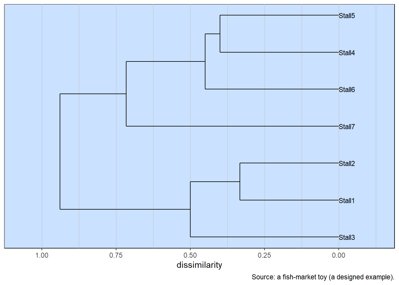
Here are the stalls, drawn from the very dissimilarity matrix we built in the last chapter.
Show the code
dissimilarity(two_way, what ="site") |>dendrogram_plot(caption = data_source)
The stalls as a tree. Stalls that join near the right keep similar stock; the two families meet only at the far left.
Read it from the right. Each stall begins as its own twig at dissimilarity zero — every stall is identical to itself. Moving left, twigs join into branches, and the height of each join is how dissimilar the two things being joined are. A join near the right is between near-twins; a join far to the left is between things that share little.
Now the structure reads itself. Stall4 and Stall5 join early, at a dissimilarity of about four-tenths — which is exactly the 0.40 they showed in the matrix. Stall6 joins them, and Stall7 attaches to that finfish branch a little further out, the half-committed mixed stall again. Below, the three shellfish stalls gather the same way. And the two clusters do not meet until the far left, near one: between the finfish stalls and the shellfish stalls there is almost nothing in common. The tree has taken the two pale blocks and the wall of ones from the heatmap and stood them up as branches.
5.2 The items
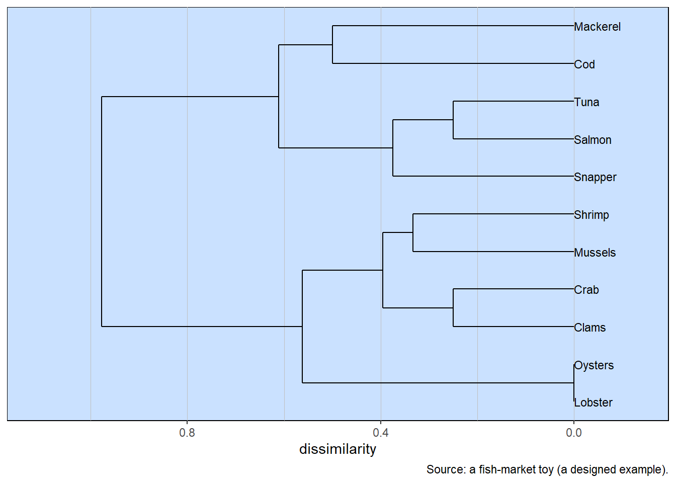
The same drawing rescues the item matrix we declined to print.
Show the code
dissimilarity(two_way, what ="item") |>dendrogram_plot(caption = data_source)
The items as a tree — the eleven-by-eleven matrix we did not print, made readable at a glance.
There are the eleven items, and the hundred and twenty-one numbers, in a shape you can take in at a breath: two families, finfish above and shellfish below, meeting only at the far left. Inside each, the tight pairs stand out — Tuna with Salmon, Oysters with Lobster, things that travel together — while Cod, sold at its single stall, hangs at the edge of the finfish branch beside Mackerel, the two loosest members of their group. Everything the matrix knew is here. It is simply legible now.
5.3 A caution worth keeping
A dendrogram is a generous thing, and that is exactly its danger. It will draw you a tree no matter what you feed it. Shuffle the data into nonsense and it still returns a tidy branching picture, because some tree can always be drawn. The eye, meanwhile, is eager to group: show a person a tree and they begin circling clusters, and they will find them whether or not the data truly supports them.
So read a dendrogram for the structure that is unmistakable, and hold the rest lightly. Here the two families are not in doubt — the gap between them is enormous and it agrees with everything else we have seen. The fine branchings near the right are another matter. Whether Tuna, Salmon, and Snapper are a cluster of three, or a pair with a near neighbour, is the kind of question the picture invites but cannot answer. How many groups there are, and where to draw their boundaries, is a decision, not a discovery. It matters enough that a later chapter is given over to making that decision carefully, with data and a rule chosen for the purpose. For now, trust the big divisions and treat the small ones as suggestions.
5.4 Two quiet choices
One last thing to notice, because it returns. To draw this tree we made two choices and mentioned neither. We chose a way to measure how dissimilar two things are — the Jaccard measure of the last chapter — and a way to decide how far apart two whole branches are when we join them. We took the obvious option for each. But they were choices, and different ones would have drawn a different tree from the very same data. The next chapter brings both into the open, because a picture that shifts with the choices behind it is an argument, not a fact, and you are better off knowing which choices you have made.