Every tree we have drawn rested on two decisions, and we made both without comment. We chose a way to measure how dissimilar two things are, and a way to decide how far apart two whole branches sit when the time comes to join them. Neither choice is forced; each has sensible alternatives; and each, changed, can change the tree. This chapter brings the two decisions into the open and watches the picture respond. The aim is not to crown one choice the right one — often several are defensible — but to show that a dendrogram is built by choices, and that an honest tree arrives with its choices stated.
Show the code
## data wrangling, tables, dendrograms, and panelslibrary(tidyverse)library(gt)library(ggdendro)library(patchwork)## the listsr package: the list -> tree + assessment-line toolkitlibrary(listsr)## the running example, read in againdata_source <-"Source: a fish-market toy (a designed example)."data_rows <-"Stall1, Mussels, Crab, Lobster, Shrimp, Oysters, Clams Stall2, Clams, Mussels, Shrimp, Crab Stall3, Oysters, Crab, Lobster, Clams Stall4, Mackerel, Cod, Tuna, Snapper, Salmon Stall5, Snapper, Tuna, Salmon Stall6, Salmon, Mackerel, Tuna Stall7, Snapper, Clams, Shrimp, Tuna"fish <-read_lists(data_rows)two_way <-data_to_2way(fish)
6.1 The first choice: how to measure distance
The dissimilarity we have used all along counts, out of every item either of two stalls sold, the fraction only one of them had. It has a name, the Jaccard measure, and it is the natural one for lists of present-or-absent things: it looks only at what is there, ignores the order, and never lets a shared absence — two stalls both not selling octopus — count as a point of resemblance. There are other measures in the same family, and for presence-and-absence data they tend to agree with one another, so this first choice is usually the quieter of the two. We will keep Jaccard and spend our attention on the second choice, which is where the picture really moves.
6.2 The second choice: how to join branches
When two single stalls join, the height of their join is simply their dissimilarity; there is nothing to decide. But the moment a branch holds two or more stalls, a new question appears with no obvious answer: how far is this branch from that one? You could measure from their nearest members, or their farthest, or take the average over all the pairs between them, or pick whichever merge least increases the spread within the new group. Each of those is a rule — called a linkage — and each is reasonable. The trouble is that they need not agree.
So let us hold the data and the distance fixed, change only the linkage, and draw the same stalls four times.
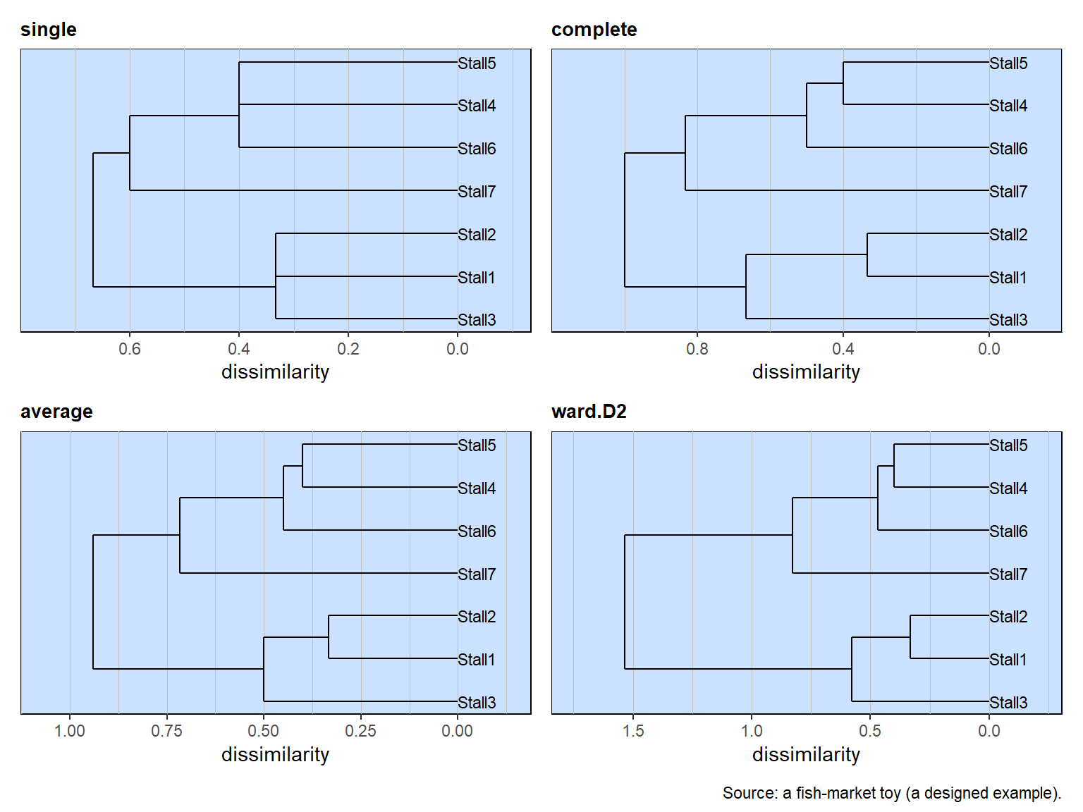
The same stalls, the same Jaccard distances, four linkage rules. The grouping holds; the ruler does not.
Look first at what does not change. In all four panels the same two families appear, with the same members, and the mixed Stall7 hangs off the finfish side every time. Who groups with whom is settled; the linkage does not touch it.
Now look at what does change: the ruler along the bottom. Single linkage joins branches by their nearest members, so every height is pulled low and the whole tree looks compact — the two families seem to meet at a dissimilarity of about two-thirds. Complete linkage measures from the farthest members and pushes the joins outward, so the families meet near one. Ward’s rule runs on a different scale altogether; read it without noticing, and you would think these stalls far more separated than the single-linkage tree says — yet it is the very same data. The linkage here sets the ruler, not the groups.
6.3 What is robust, and what is not
That the grouping survived all four rules is reassuring, and it is not guaranteed. Here the two families are so cleanly separated that no reasonable choice can pull them apart. Run the same comparison on the eleven items and the headline holds — finfish and shellfish stay distinct under every linkage — but the fine structure inside each family shifts: which shellfish pairs first, where Cod and Mackerel finally settle. The strong division is robust; the small ones are partly the rule talking.
That gives a plain working test, and it is the most useful thing in this chapter. A pattern you can trust is one that holds up when you change the choices behind it. A grouping that appears under one linkage and dissolves under the next was never really in the data — it was in the rule. So vary the choices on purpose, and keep what survives.
6.4 The procedure, not the picture
A dendrogram persuades precisely because it hides its own making. The branches look like facts of nature, when they are the output of a measure you picked and a linkage you picked, run on the data you happened to collect. None of that makes the tree untrue — it makes it conditional, and the remedy is simple honesty: state the distance, state the linkage, prefer what is robust to both, and remember that the tree answers the exact question you posed in the exact way you posed it.
Two questions are left over, and they shape the chapters ahead. Does anything outside these lists agree with the grouping the tree proposes? That is the next chapter, where we bring in what we know about the stalls themselves. And where, precisely, do the groups begin and end — not by eye, and not by fiat, but by a rule we can defend? That is the chapter after, and we will answer it with discipline rather than a confident wave at the picture.