library(ggplot2)
library(dplyr)
library(tidyr)
library(patchwork) # For combining plots
# 1. Setup Data (Cleaned & Accurate)
# We will filter out NAs for the calculation to be accurate
data_raw <- tribble(
~Year, ~Company, ~Hex,
2026, "Pantone", "#F0EEE9", 2026, "Benj. Moore", "#4A413C", 2026, "Sherwin", "#BCA68E", 2026, "Behr", "#6A867F", 2026, "Valspar", "#7A8B78", 2026, "Dunn-Edw", "#2E4035", 2026, "Glidden", "#9D4A3C",
2025, "Pantone", "#A47864", 2025, "Benj. Moore", "#AA8C96", 2025, "Sherwin", "#A3AF9D", 2025, "Behr", "#8A3324", 2025, "Valspar", "#2C5282", 2025, "Dunn-Edw", "#B58463", 2025, "Glidden", "#6A4B5F",
2024, "Pantone", "#FFBE98", 2024, "Benj. Moore", "#5B6C91", 2024, "Sherwin", "#B4BEC3", 2024, "Behr", "#4E5052", 2024, "Valspar", "#97C5C9", 2024, "Dunn-Edw", "#7DA6B3", 2024, "Glidden", "#EFDECD",
2023, "Pantone", "#BE3455", 2023, "Benj. Moore", "#D25A46", 2023, "Sherwin", "#AE8E7E", 2023, "Behr", "#F0ECE2", 2023, "Glidden", "#3A6A6C", 2023, "Dunn-Edw", "#A66E6A",
2022, "Pantone", "#6667AB", 2022, "Benj. Moore", "#A3AA9E", 2022, "Sherwin", "#95978A", 2022, "Behr", "#B8CBC0", 2022, "Glidden", "#8C9C74", 2022, "Dunn-Edw", "#947B64",
2021, "Pantone", "#C4BA4E", 2021, "Benj. Moore", "#647882", 2021, "Sherwin", "#545E60", 2021, "Behr", "#C09277", 2021, "Glidden", "#D0C5B3", 2021, "Dunn-Edw", "#7D8F9E",
2020, "Pantone", "#0F4C81", 2020, "Benj. Moore", "#EBE1E1", 2020, "Sherwin", "#2F3D4C", 2020, "Behr", "#97A878", 2020, "Glidden", "#304B64", 2020, "Dunn-Edw", "#B6E0D2",
2019, "Pantone", "#FF6F61", 2019, "Benj. Moore", "#AFB4B4", 2019, "Sherwin", "#D1866A", 2019, "Behr", "#4D6C8C", 2019, "Glidden", "#004746", 2019, "Dunn-Edw", "#8D4E3C",
2018, "Pantone", "#5F4B8B", 2018, "Benj. Moore", "#AF2D2D", 2018, "Sherwin", "#195564", 2018, "Behr", "#7E9995", 2018, "Glidden", "#202226", 2018, "Dunn-Edw", "#3D4F46",
2017, "Pantone", "#88B04B", 2017, "Benj. Moore", "#5F505F", 2017, "Sherwin", "#8C827D", 2017, "Behr", "#D5CDB5", 2017, "Glidden", "#7A5C6D", 2017, "Dunn-Edw", "#E3B668",
2016, "Pantone", "#C4B9D0", 2016, "Benj. Moore", "#F3F4ED", 2016, "Sherwin", "#EDEAE0", 2016, "Glidden", "#7B9683"
)
# 2. Extract RGB & Luminance
get_vals <- function(hex) {
rgb <- col2rgb(hex)
# Standard Luminance formula (Perceived Brightness)
lum <- (0.299 * rgb[1] + 0.587 * rgb[2] + 0.114 * rgb[3])
c(R = rgb[1], G = rgb[2], B = rgb[3], Lum = lum)
}
df_vals <- cbind(data_raw, t(sapply(data_raw$Hex, get_vals)))
# 3. ANALYSIS A: CONSENSUS (Dispersion)
# Calculate the "Centroid" (Average Color) of each year, then avg distance from it
df_dispersion <- df_vals %>%
group_by(Year) %>%
summarise(
Mean_R = mean(R), Mean_G = mean(G), Mean_B = mean(B)
) %>%
inner_join(df_vals, by = "Year") %>%
mutate(
dist_from_mean = sqrt((R - Mean_R)^2 + (G - Mean_G)^2 + (B - Mean_B)^2)
) %>%
group_by(Year) %>%
summarise(Dispersion = mean(dist_from_mean))
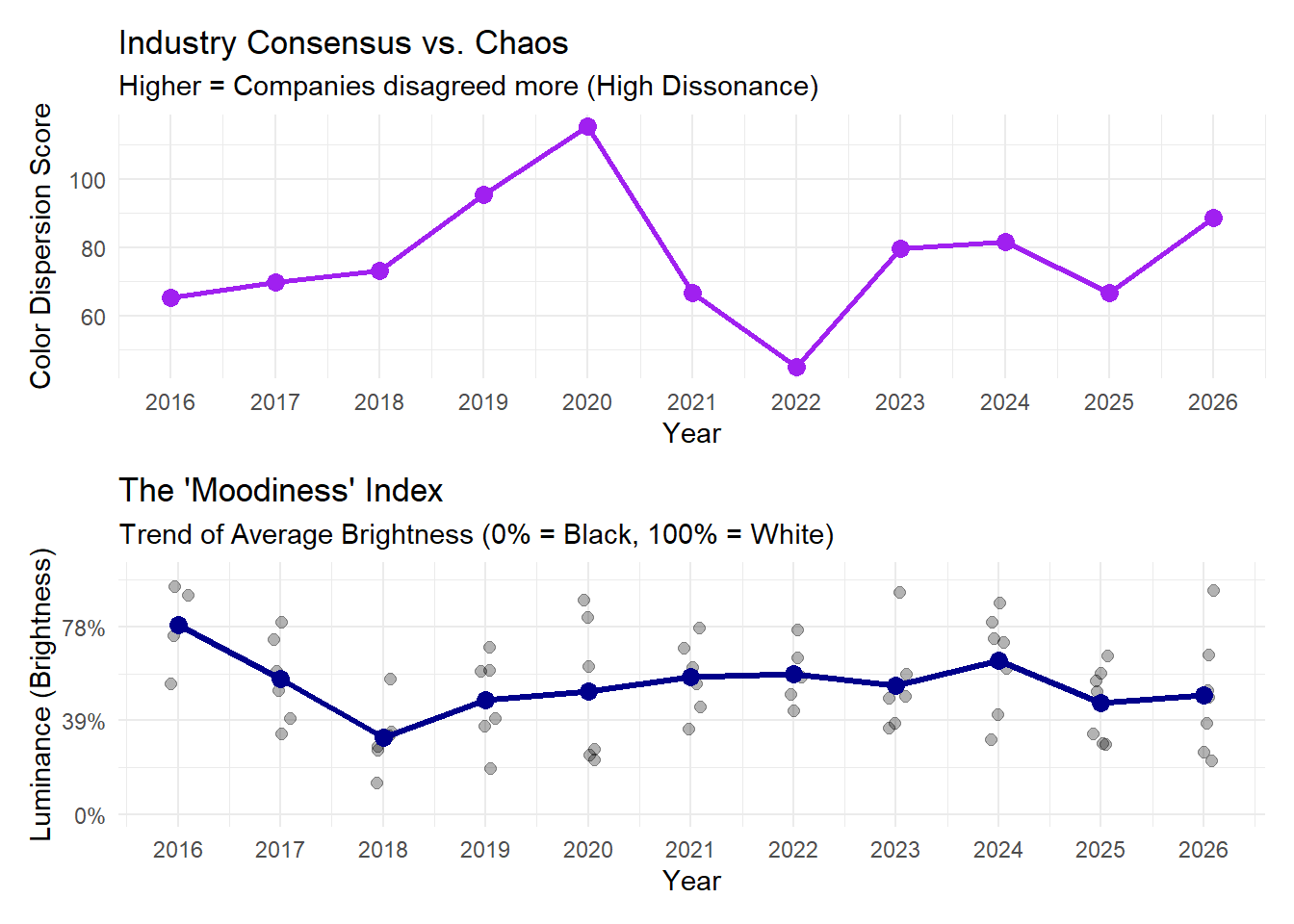
# Plot A: The "Confusion" Chart
p1 <- ggplot(df_dispersion, aes(x = Year, y = Dispersion)) +
geom_line(color = "purple", size = 1) +
geom_point(size = 3, color = "purple") +
scale_x_continuous(breaks = 2016:2026) +
labs(title = "Industry Consensus vs. Chaos",
subtitle = "Higher = Companies disagreed more (High Dissonance)",
y = "Color Dispersion Score") +
theme_minimal()
# 4. ANALYSIS B: LUMINANCE (Moodiness)
# Plot B: The "Light vs Dark" Chart
p2 <- ggplot(df_vals, aes(x = Year, y = Lum)) +
# Add individual points
geom_jitter(width = 0.1, size = 2, alpha = 0.3) +
# Add trend line (Mean Luminance)
stat_summary(fun = mean, geom = "line", color = "darkblue", size = 1.2, group = 1) +
stat_summary(fun = mean, geom = "point", color = "darkblue", size = 3) +
scale_x_continuous(breaks = 2016:2026) +
scale_y_continuous(limits = c(0, 255), labels = function(x) paste0(round(x/2.55), "%")) +
labs(title = "The 'Moodiness' Index",
subtitle = "Trend of Average Brightness (0% = Black, 100% = White)",
y = "Luminance (Brightness)") +
theme_minimal()
# Combine plots (Requires 'patchwork' library)
p1 / p2