# Load necessary libraries
if (!require("dendextend")) install.packages("dendextend")
if (!require("dplyr")) install.packages("dplyr")
if (!require("colorspace")) install.packages("colorspace")
library(dendextend)
library(dplyr)
library(colorspace)
# Suppress startup messages
suppressPackageStartupMessages(library(dendextend))
# 1. Setup the Full Data
# (Aggregating all our cleaned data points)
data_raw <- tribble(
~Year, ~Company, ~Name, ~Hex,
2026, "Pantone", "Cloud Dancer", "#F0EEE9",
2026, "BM", "Silhouette", "#4A413C",
2026, "SW", "Univ. Khaki", "#BCA68E",
2026, "Behr", "Hidden Gem", "#6A867F",
2026, "Valspar", "Warm Eucalyptus", "#7A8B78",
2026, "Dunn", "Midnight Garden", "#2E4035",
2026, "Glidden", "Warm Mahogany", "#9D4A3C",
2025, "Pantone", "Mocha Mousse", "#A47864",
2025, "BM", "Cinnamon Slate", "#AA8C96",
2025, "SW", "Quietude", "#A3AF9D",
2025, "Behr", "Rumors", "#8A3324",
2025, "Valspar", "Encore", "#2C5282",
2025, "Dunn", "Caramelized", "#B58463",
2024, "Pantone", "Peach Fuzz", "#FFBE98",
2024, "BM", "Blue Nova", "#5B6C91",
2024, "SW", "Upward", "#B4BEC3",
2024, "Behr", "Cracked Pepper", "#4E5052",
2024, "Valspar", "Renew Blue", "#97C5C9",
2024, "Dunn", "Skipping Stones", "#7DA6B3",
2023, "Pantone", "Viva Magenta", "#BE3455",
2023, "BM", "Raspberry Blush", "#D25A46",
2023, "SW", "Redend Point", "#AE8E7E",
2023, "Behr", "Blank Canvas", "#F0ECE2",
2023, "Dunn", "Terra Rosa", "#A66E6A",
2022, "Pantone", "Very Peri", "#6667AB",
2022, "BM", "October Mist", "#A3AA9E",
2022, "SW", "Evergreen Fog", "#95978A",
2022, "Behr", "Breezeway", "#B8CBC0",
2022, "Dunn", "Art & Craft", "#947B64",
2021, "Pantone", "Ult. Gray", "#939597",
2021, "BM", "Aegean Teal", "#647882",
2021, "SW", "Urbane Bronze", "#545E60",
2021, "Behr", "Canyon Dusk", "#C09277",
2021, "Dunn", "Wild Blue", "#7D8F9E",
2020, "Pantone", "Classic Blue", "#0F4C81",
2020, "BM", "First Light", "#EBE1E1",
2020, "SW", "Naval", "#2F3D4C",
2020, "Behr", "Back to Nature", "#97A878",
2020, "Dunn", "Minty Fresh", "#B6E0D2",
2019, "Pantone", "Living Coral", "#FF6F61",
2019, "BM", "Metropolitan", "#AFB4B4",
2019, "SW", "Cavern Clay", "#D1866A",
2019, "Behr", "Blueprint", "#4D6C8C",
2019, "Dunn", "Spice of Life", "#8D4E3C",
2018, "Pantone", "Ultra Violet", "#5F4B8B",
2018, "BM", "Caliente", "#AF2D2D",
2018, "SW", "Oceanside", "#195564",
2018, "Behr", "In The Moment", "#7E9995",
2017, "Pantone", "Greenery", "#88B04B",
2017, "BM", "Shadow", "#5F505F",
2017, "SW", "Poised Taupe", "#8C827D",
2017, "Behr", "Comfortable", "#D5CDB5",
2016, "Pantone", "Rose Quartz", "#F7CAC9",
2016, "BM", "Simply White", "#F3F4ED",
2016, "SW", "Alabaster", "#EDEAE0"
)
# 2. Prepare the Matrix for Clustering
# Extract RGB values
rgb_matrix <- t(col2rgb(data_raw$Hex))
rownames(rgb_matrix) <- paste(data_raw$Year, data_raw$Company, data_raw$Name, sep = " - ")
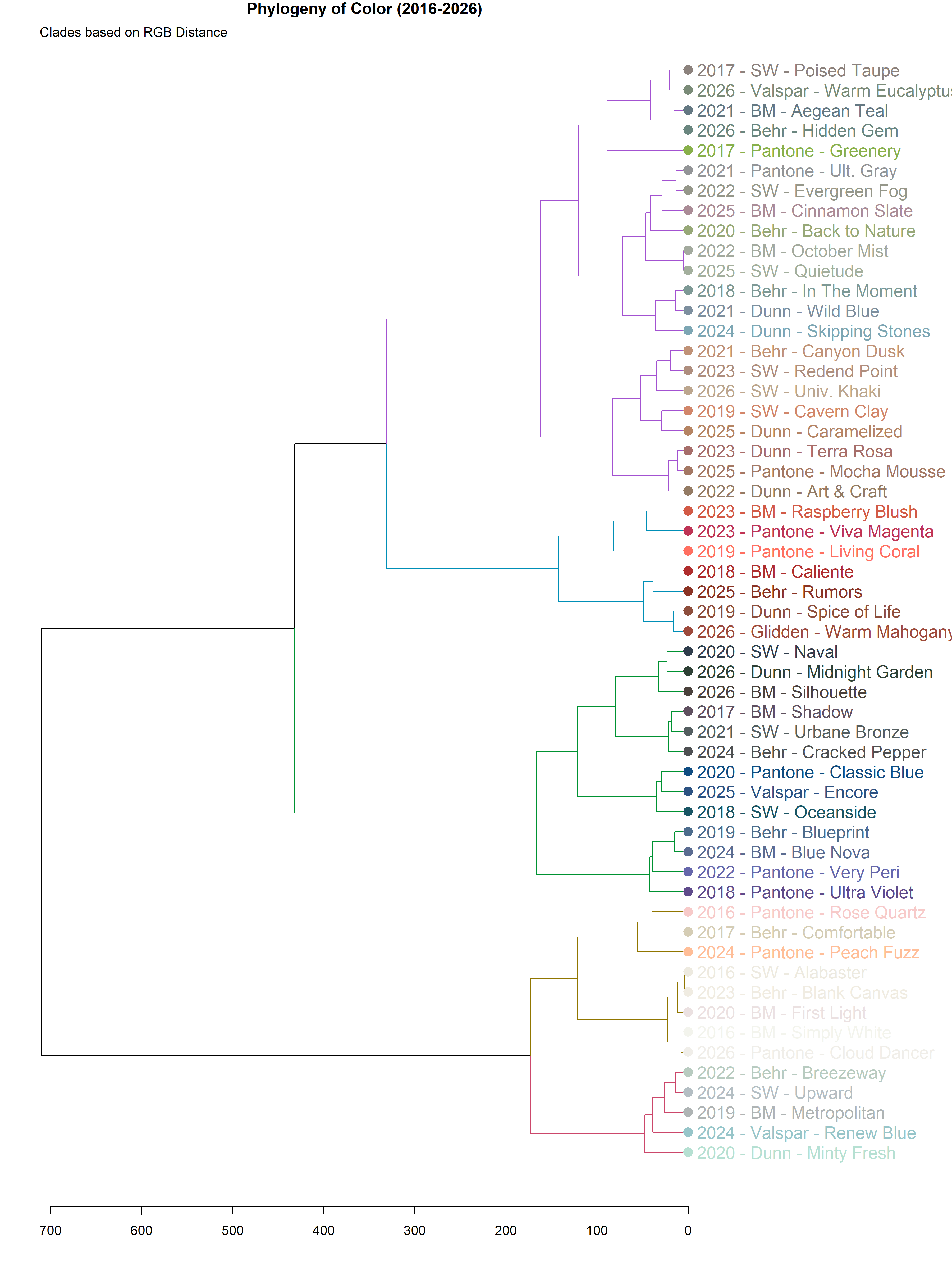
# 3. Hierarchical Clustering (The "Phylogeny")
# Method: Ward.D2 (Minimizes variance within clusters, good for "species" grouping)
d_matrix <- dist(rgb_matrix, method = "euclidean")
hc <- hclust(d_matrix, method = "ward.D2")
# 4. Create Dendrogram Object
dend <- as.dendrogram(hc)
# ... (Keep your existing data_raw and clustering code from step 1-4) ...
# 5. Assign Colors (Same as before)
labels_order <- labels(dend)
color_lookup <- setNames(data_raw$Hex, paste(data_raw$Year, data_raw$Company, data_raw$Name, sep = " - "))
leaf_colors <- color_lookup[labels_order]
# 6. Formatting the Dendrogram
dend <- dend %>%
set("labels_col", leaf_colors) %>%
set("labels_cex", 1.3) %>% # Adjust text size
set("branches_k_color", k = 5) %>%
set("leaves_pch", 19) %>%
set("leaves_col", leaf_colors) %>%
set("leaves_cex", 1.5) # Slightly larger colored dots
# 7. EXPORT TO FILE (The "Expansion" Fix)
# We set height = 1200 to stretch the y-axis
png(filename = "color_phylogeny_tall.png", width = 3600, height = 4800, res = 300)
# Adjust margins: Bottom, Left, Top, Right (Increase Right for long names)
par(mar = c(4, 1, 1, 15))
# Plot horizontally
plot(dend, horiz = TRUE, main = "Phylogeny of Color (2016-2026)")
# Add Legend
legend("topleft", legend = "Clades based on RGB Distance", bty = "n", cex = 1.0)
# Close the file
dev.off()
# Confirmation message
print("Plot saved as 'color_phylogeny_tall.png' in your working directory.")