1  Start with Photos

Cell-phone photos contain valuable information besides the image. Date, time, and location coordinates are the important metadata elements used here.

Limitations

This has been tested only with Android phone photos. The processing was done with RStudio in a Windows 11 environment. The LLM model is OpenAI 4o.

1.1 Setup & Initialize

The usual processing to get the libraries and data ready.

## Standard Libraries
library(readr)        ## Read in data
library(stringi)      ## String functions, incl stri_wrap
library(ggmap)        ## Show maps, handle Google key
library(ggplot2)      ## Build chart & maps
library(dplyr)        ## General data wrangling
library(gt)           ## Tables
library(here)         ## Directory simplification


## Specialized Libraries
library(lubridate)    ## Times and dates
library(exifr)        ## Get photo EXIF data
library(grobblR)      ## Arrange photos
library(jpeg)         ## Handle jpeg images
library(png)          ## Hangle png images
library(magick)       ## Manipulate images
library(ggpubr)       ## Arrange photos
library(numbers)      ## Mod function
library(pdftools)     ## Good help with PDFs

## Packages from github/kimbridges
## install_github("kimbridges/sitemaps")
library(sitemaps)

## OpenAI Access
library(accessOAI)

## Get API Keys
apiKey <- Sys.getenv("OPENAI_API_KEY")

googleKey <- Sys.getenv("GGMAP_GOOGLE_API_KEY")
register_google(key = googleKey, account_type = "standard")

## Some standard setup
## Use two functions from sitemaps to initialize parameters
column <- site_styles()
hide  <- site_google_hides()

## Establish a theme that improves the appearance of a map.
## This theme removes the axis labels and 
## puts a border around the map. No legend.
simple_black_box <- theme_void() +
              theme(panel.border = element_rect(color = "black", 
                                   fill=NA, 
                                   size=2),
                    legend.position = "none")

1.2 Get a Set of Photos

The assumption is that you have taken photos each day that document each of your activities. Generally, you’ll have multiple photos of each place you’ve stopped and what you did at each place.

Your photos are stored on your cell phone. They are likely backed up on the cloud, too. Using the cloud storage photo tool provided by Google (photos.google.com) is a handly way to review the set of photos. However, these clould images don’t have all the EXIF data (e.g., they are missing the geographic coordinates). Therefore, we can’t use them directly. Instead, we need to transfer some stored files to the computer.

Probably the most straightforward way to move your files is with Google’s takeout service. You can also move photos from a phone with a cable connection. This isn’t as practical if you’ve stored thousands of photo on your phone.

A step-by-step procedure for using Google Takeout is given in the Appendix.

1.3 Create Some Folders

The first step is to create a file structure so that the results of the computations are put into logical locations. This makes it straightforward to process different folders with sets of photos without co-mingling or overwriting objects from previous uses of the procedures.

Note that only the “source” and “folder” (where the photos are kept) are provided. With a tiny exception in the mapping done in the Data Grouping chapter, no other input is required.

### Input Area ########################################

## Source information to label visualizations.
source <- "Europe 2024"

## Location of the photos for the day.
folder <- "photos/day_03"

######################################################

## Test if the 'files' and 'thumbs' folders exist.
thumbs_folder <- paste0(folder,"/thumbs")
thumbs_test   <- file.exists(thumbs_folder)
files_folder  <- paste0(folder,"/files")
files_test    <- file.exists(files_folder)

## Create 'files' and 'thumbs' folders if they don't exist.
if(isFALSE(thumbs_test)){
  dir.create(file.path(folder, "thumbs"), 
             showWarnings = FALSE)
}

if(isFALSE(files_test)){
  dir.create(file.path(folder, "files"), 
             showWarnings = FALSE)
}

## Write a file that links to file names.
## This is needed to communicate between chapters.
baseinfo <- NULL
baseinfo$source <- source
baseinfo$folder <- folder
baseinfo$thumbs_folder <- thumbs_folder
baseinfo$files_folder <- files_folder
baseinfo <- as.data.frame(baseinfo)

write.table(baseinfo, file="baseinfo.txt")

1.4 Extract Photo Metadata

The metadata include the date and time each photo was taken, as well as the geographic coordinates of the location.

The values are extracted, formatted and saved into a file that will grow with new data columns as more and more information is obtained.

This processing step includes a reverse geocoding step. This computation provides the geographic coordinates to the Google Map API. The result is the name of the location, from the street address to the country.

## Read all the file names in the folder.
files <- list.files(path=here(folder), 
                    pattern="*.jpg", 
                    full.names=TRUE, 
                    recursive=FALSE)

## Count the photos in the folder.
no_files <- length(files)

## Initialize the table to hold the data.
table_info <- setNames(data.frame(matrix(ncol = 5, nrow = 0)), 
              c("number", "file", "location", "date", "time"))

## Specify which attributes of the EXIF to read.
  tags <- c("GPSLatitude","GPSLongitude","DateTimeOriginal")

## Process the photos, one at a time.
for (i in 1:no_files){
 
  ## Here is where the heavy lifting is done.
  sheet  <- image_read(files[i])
  
  ## Extract the EXIF info.
  photo_exif <- read_exif(path=files[i],
                          tags=tags,
                          recursive = FALSE)

  ## Make a small, reference image.
  small_photo <- magick::image_scale(sheet,"10%")

  ## Get the location and put in easy-to-use variables.
  img_lat <- photo_exif$GPSLatitude
  img_lon <- photo_exif$GPSLongitude
  img_location <- c(img_lon, img_lat)
  
  ## Process the date and time.
  img_date <- as.Date(substring(photo_exif$DateTimeOriginal,1,10),
                     "%Y:%m:%d")
  lub_str   <- ymd_hms(photo_exif$DateTimeOriginal) 
  img_hour   <- hour(lub_str)
  img_minute <- minute(lub_str)
  img_minute <- sprintf("%02d",img_minute)
  img_time   <- paste0(img_hour,":",img_minute)
  img_date <- as.Date(substring(photo_exif$DateTimeOriginal,1,10),
                     "%Y:%m:%d")
  img_when <- paste0(img_time," on ",weekdays(img_date),", ",
                    format(img_date, format="%B %d, %Y")) 

  ## Get the name of the place (wrap, if necessary).
  img_place_name <- revgeocode(img_location)
  img_place_name <- stri_wrap(img_place_name, width = 50)
  
  ## Caption with place name and when the photo was taken.
  place_caption <- paste0("Photo: ",i," -- ", 
                          img_when,"\n",img_place_name[1])

  ## Composite the image and the caption.
  out_img <- image_ggplot(small_photo)
  out_img <- out_img + ggtitle(place_caption) +
    theme_bw() +
    theme(axis.line=element_blank(),
      axis.text=element_blank(),
      axis.ticks=element_blank(),
      axis.title=element_blank())
 
  ## Write the labeled thumbnail to a file.
  thumb_name <- paste0(thumbs_folder,"/photo_",i,".png")
  ggsave(thumb_name,out_img)
  
  ## Build a table row with image data.
  f_name <- basename(files[i])
  table_list <- data.frame(number=i, 
                           file = f_name, 
                           location=img_place_name[1], 
                           date=img_date, 
                           time=img_time,
                           lat = img_lat,
                           lon = img_lon)
  
  ## Add the row to the table.
  table_info <- rbind(table_info, table_list)

 } ## End photo loop

## Save the table for later use.
file_location <- paste0(files_folder,"/photo_info.txt")
write.table(table_info,
            file = file_location)

1.5 Print an Information Table

It’s good to look at the results of the processing.

The data for each photo is sufficiently long that the table is divided into two parts.

Future Task: Save these tables as PDF files.

## Read data about the photos.
file_location <- paste0(files_folder,"/photo_info.txt")
table_info <- read.table(file = file_location)

## Break the table into two parts.
left_part <- table_info |>
  select(number:location)
right_part <- table_info |>
  select(number, date:lon)

## Create a table (in two parts) with the photo information.
table_1 <- gt(left_part) %>% 
  tab_header(
    title = paste0("Photo Index (part 1): ", folder)
    ) %>% 
  tab_source_note(
    source_note = paste0("Report Prepared: ",Sys.Date())
  ) %>%
  tab_style(
    style = cell_text(v_align="top"),
    locations = cells_body()
    ) %>% 
  opt_row_striping(row_striping = TRUE)

table_1

Photo Index (part 1): photos/day_03
number	file	location
1	PXL_20240503_074028210.jpg	Pelikaanstraat 1/100, 2018 Antwerpen, Belgium
2	PXL_20240503_095732068.MP.jpg	Tuinstraat 26, 2613 RC Delft, Netherlands
3	PXL_20240503_101931305.MP.jpg	Koningin Julianalaan 10, 2595 AA Den Haag,
4	PXL_20240503_104015795.jpg	Gravenstraat 5, 2513 AK Den Haag, Netherlands
5	PXL_20240503_105530439.jpg	Hoogstraat 2, 2513 AR Den Haag, Netherlands
6	PXL_20240503_131556568.MP.jpg	Korte Vijverberg 8, 2513 AB Den Haag, Netherlands
7	PXL_20240503_131800759.MP.jpg	Plein 29, 2511 CS Den Haag, Netherlands
8	PXL_20240503_134649910.MP.jpg	Korte Vijverberg 8, 2513 AB Den Haag, Netherlands
9	PXL_20240503_141041338.jpg	Binnenhof 17, 2513 AA Den Haag, Netherlands
10	PXL_20240503_141233240.jpg	Binnenhof 11, 2513 AA Den Haag, Netherlands
11	PXL_20240503_142647554.jpg	Gravenstraat 2, 2513 AK Den Haag, Netherlands
12	PXL_20240503_153252185.jpg	Denneweg 130, 2514 CL Den Haag, Netherlands
13	PXL_20240503_154539276.jpg	Denneweg 130, 2514 CL Den Haag, Netherlands
14	PXL_20240503_162546980.jpg	Denneweg 130, 2514 CL Den Haag, Netherlands
15	PXL_20240503_173611221.jpg	Denneweg 130, 2514 CL Den Haag, Netherlands
16	PXL_20240503_174951419.jpg	Denneweg 126A, 2514 CL Den Haag, Netherlands
Report Prepared: 2024-06-10

table_2 <- gt(right_part) %>% 
  tab_header(
    title = paste0("Photo Index (part 2): ", folder)
    ) %>% 
  tab_source_note(
    source_note = paste0("Report Prepared: ",Sys.Date())
  ) %>%
  tab_style(
    style = cell_text(v_align="top"),
    locations = cells_body()
    ) %>% 
  opt_row_striping(row_striping = TRUE)

table_2

Photo Index (part 2): photos/day_03
number	date	time	lat	lon
1	2024-05-03	9:40	51.21683	4.421017
2	2024-05-03	11:57	52.00732	4.353553
3	2024-05-03	12:19	52.08117	4.323594
4	2024-05-03	12:40	52.07826	4.309892
5	2024-05-03	12:55	52.07822	4.309008
6	2024-05-03	15:15	52.08040	4.314497
7	2024-05-03	15:18	52.08031	4.314269
8	2024-05-03	15:46	52.08027	4.314536
9	2024-05-03	16:10	52.08034	4.314133
10	2024-05-03	16:12	52.07986	4.313383
11	2024-05-03	16:26	52.07827	4.309814
12	2024-05-03	17:32	52.08585	4.311544
13	2024-05-03	17:45	52.08585	4.311542
14	2024-05-03	18:25	52.08586	4.311558
15	2024-05-03	19:36	52.08585	4.311556
16	2024-05-03	19:49	52.08590	4.311847
Report Prepared: 2024-06-10

1.6 Create Photo Sheets

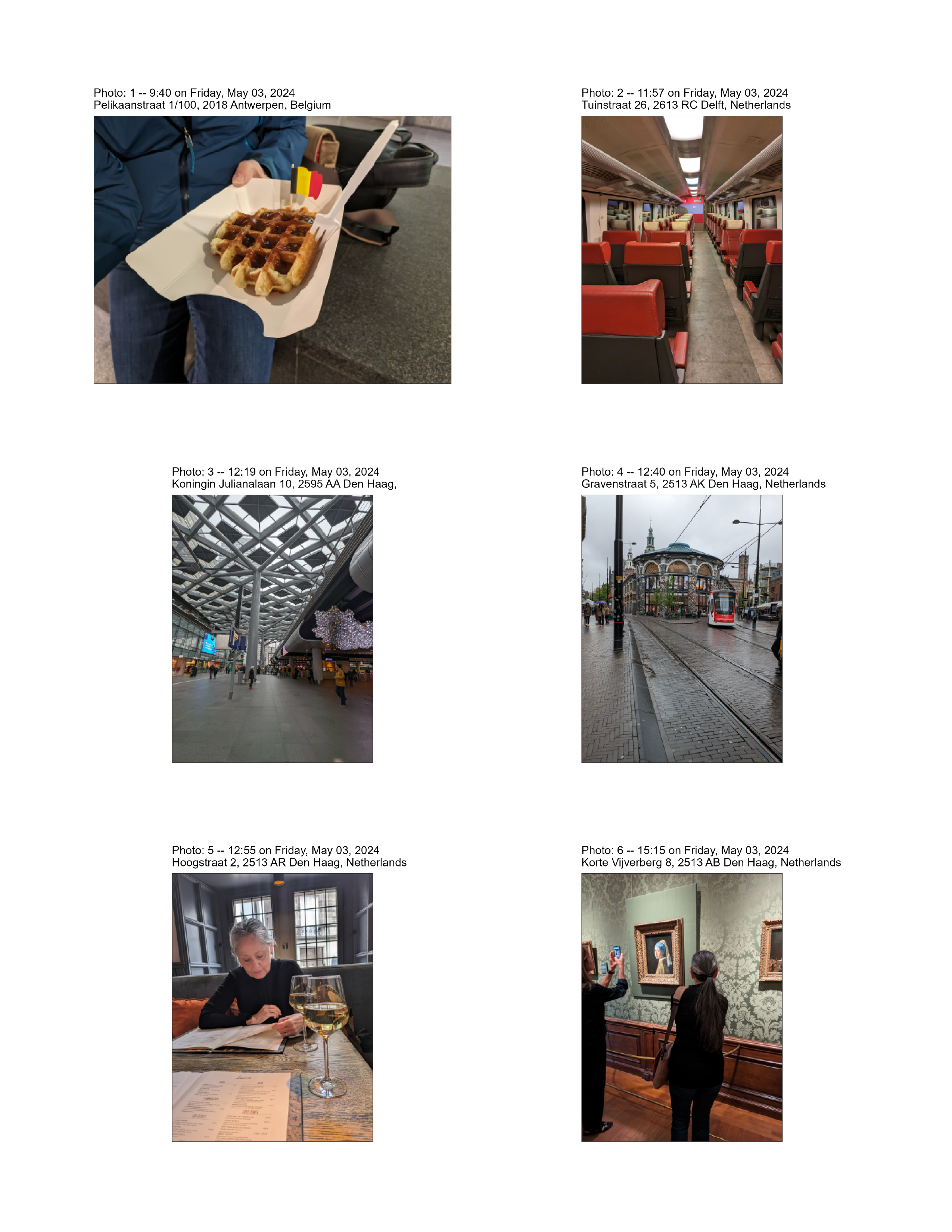
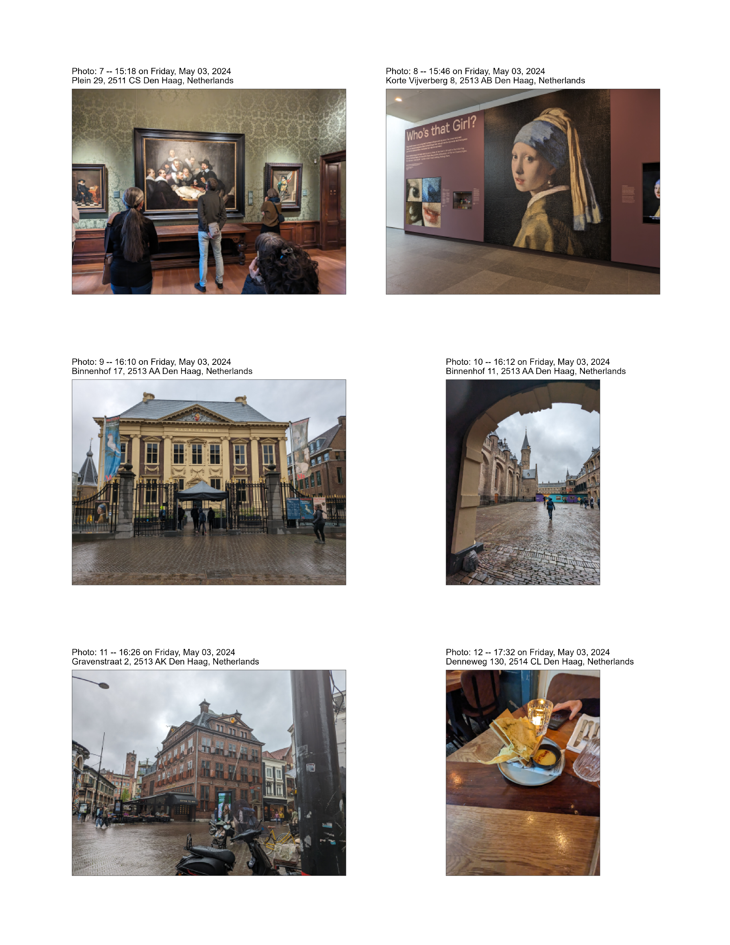
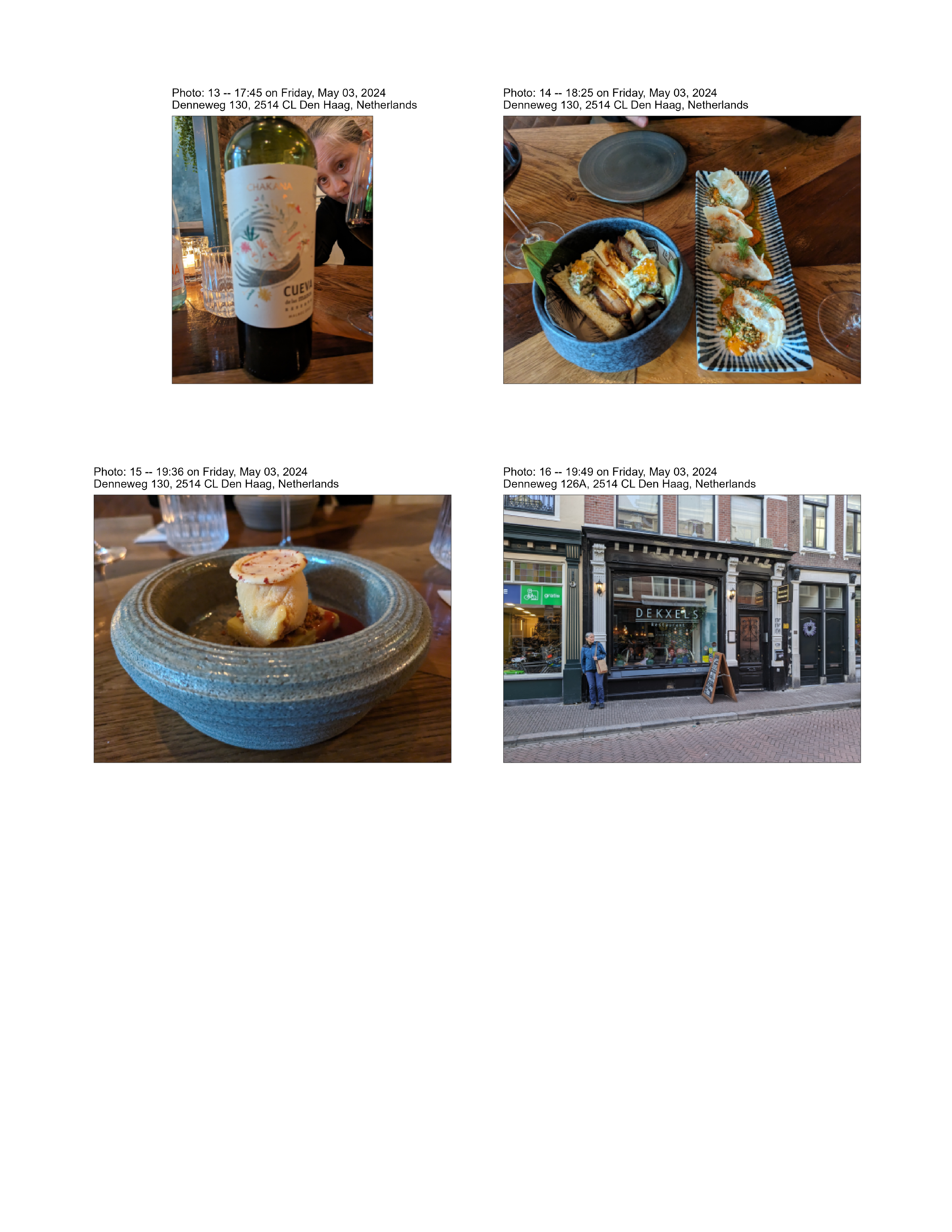
Photo sheets show thumbnail images of the photos, along with captions with the date, time and location of the photo.

Future Task: Place the LLM-generated caption (see Image Interpretation chapter) on each thumbnail.

## Create a blank image and save it.
## This is used later when images are printed.
blank <- magick::image_blank(width=640, height=480, 
                             color = "white", 
                             ##pseudo_image = "", 
                             defines = NULL)
blank_location <- paste0(files_folder,"/z_blank.png")
magick::image_write(image=blank,path=blank_location)

## Get a list of the photos, including the photo names.
file_location <- paste0(files_folder,"/photo_info.txt")
photo_list <- read.table(file = file_location)

## Number of photos.
n_photos <- nrow(photo_list)

## Round the number of files up to a multiple of 6
files_ceiling <- ceiling(n_photos/6) * 6

## Process each labeled small picture, one at a time
page_no <- 0

for(i in 1:files_ceiling){

## Up to six images per page
  ## Count by six
  img_no <- mod(i-1,6) + 1
 
  ## Build a name for the temporary grob image
  img_name <- paste0(thumbs_folder,"/photo_",i,".png")
  if(!file.exists(img_name))img_name <- blank_location

  if(img_no == 1) img1g <- grob_image(img_name)
  if(img_no == 2) img2g <- grob_image(img_name)
  if(img_no == 3) img3g <- grob_image(img_name)
  if(img_no == 4) img4g <- grob_image(img_name)
  if(img_no == 5) img5g <- grob_image(img_name)
  if(img_no == 6) img6g <- grob_image(img_name)
  
  ## Things to do when the images fill a page
  if(img_no == 6){
    
    ## Keep track of the page count
    page_no <- page_no + 1
    
    ## Make a montage
    page <- grob_layout(
      grob_row(
        grob_col(img1g),
        grob_col(img2g)
        ),
      grob_row(
        grob_col(img3g),
        grob_col(img4g)
        ),
      grob_row(
        grob_col(img5g),
        grob_col(img6g)
        ),
      height = 279.4, 
      width = 215.9)   

    ## File name for the PDF & PNG files.
    pdf_name <- paste0(files_folder,
                       "/page_",page_no,".pdf")
    png_name <- paste0(files_folder,
                       "/page_",page_no,".png")

    ## Put the page into a PDF file.
    grob_to_pdf(
      list(page),
      file_name = pdf_name)
      ##meta_data_title = paste0("page_",page_no))
    
    ## Make the PDF page into a PNG file.
    bitmap <- pdf_render_page(pdf_name, 
                              page = 1, 
                              dpi = 300)
    
    ## Output the PNG file.
    png::writePNG(bitmap, png_name)
    
    } ## end img_no section

  } ## end for loop

## Remove the blank image.
file.remove(blank_location)

[1] TRUE

1.7 Show photo sheets

The photo sheets are stored. Here is where they get put into the document.

####### NOT WORKING

## How many sheets.
sheets <- list.files(path=files_folder, 
                    pattern="*.png", 
                    full.names=TRUE, 
                    recursive=FALSE)

n_sheets <- length(sheets)
for (i in 1:n_sheets) {
     page_image <- sheets[i]
     page_file <- paste0("![](",
                         page_image,")\n\n")
     ##cat(":::\n")
     ##cat(page_file)
     ##cat(":::\n\n")
}

As an expedient, the pages are added manually.