We now have everything a place broadcasts: a temperature channel, a daylength channel, and a rainfall channel that knows when it’s telling the truth. The work of this chapter is to put them together. Out of three continuous numbers we want a small set of named kinds of seasonality, the cue regimes, so that we can say of a place not just how seasonal it is but what kind of seasonal it is.
A word on what these categories are, and are not. A regime is a construct, not a discovery waiting in the data. We draw the lines; the data don’t draw them for us. What makes the lines honest is that they are set by a stated rule, written down and applied the same way to every place, rather than by eye. Run the rule again and you get the same regimes. That reproducibility is the whole value of the scheme, and it’s the same principle that runs through the grouping work this project grew out of: the categories are reproducible, not proven, and they earn their keep by what they let us see.
Show the code
## --- Standard packages ---## many useful functions (dplyr, ggplot2, readr, tibble, purrr, tidyr)library(tidyverse)## formatted tableslibrary(gt)## --- Packages from github/kimbridges ---## install once with: remotes::install_github("kimbridges/seasonalityr")library(seasonalityr)## --- Options and defaults ---## suppress read_csv() column-type messagesoptions(readr.show_col_types =FALSE)## data source, cited under every tablesource <-"Monthly normals from WorldClim 2.1 (10 arc-minute), via seasonalityr."
5.1 A rule, not a black box
The classifier is classify_v2(), and its logic is a short decision the reader can follow. It works in three steps.
It starts with the rainfall channel, gated by the water balance from Chapter 4. If a place is in deficit and gets almost no rain, the rainfall channel is switched off as a mirage and the place is hyper-arid. If it’s in deficit but does get rain, that rain is reactive, a trigger. If it’s in surplus and the rain is clearly seasonal, the rain is predictive, a clock. Otherwise the rainfall channel is effectively flat, or aseasonal.
Then it reads the strength of the other two channels: whether the temperature swing is strong, moderate, or weak, and the same for daylength. A high-latitude coast with a mild temperature swing but a large daylength swing is the case that needs both.
Finally it combines them into a regime. A reactive-rain place is a desert. A predictive-rain place in the warm tropics is a wet-dry monsoon climate; the same predictive rain reinforced by a strong temperature swing is a continental summer-rain climate. An aseasonal-rain place carried by temperature alone is continental; carried by daylength alone, on a mild ocean coast, it’s maritime; carried by nothing, near the equator, it’s cue-poor. Mediterranean climates are pulled out by their winter-timed rain. The thresholds that separate strong from weak, or arid from sufficient, are fixed numbers stated in the package, not adjusted from place to place.
5.2 Running the classifier
One call does it. We take the city index table, add the daylength channel, and classify.
Show the code
## the 21-city index table (bundled), plus the daylength channelidx <-read_csv("data/cities_indices.csv") |>add_daylength()## assign each city a cue regime by the stated ruleregimes <-classify_v2(idx)## the cities grouped by the regime they fall intoregimes |>mutate(regime =factor(regime, levels =names(regime_palette()))) |>arrange(regime, name) |>select(regime, name, Tamp, SI, daylamp, m_mean) |>gt(groupname_col ="regime") |>fmt_number(columns =c(Tamp, SI, daylamp, m_mean), decimals =2) |>tab_header(title ="Twenty-one cities, sorted into cue regimes") |>tab_footnote(footnote ="Temperature channel: half the annual range, °C.",locations =cells_column_labels(columns = Tamp)) |>tab_footnote(footnote ="Rainfall channel: Walsh-Lawler seasonality index.",locations =cells_column_labels(columns = SI)) |>tab_footnote(footnote ="Daylength channel: half the annual photoperiod range, hours.",locations =cells_column_labels(columns = daylamp)) |>tab_footnote(footnote ="Water balance: mean monthly P - 2T.",locations =cells_column_labels(columns = m_mean)) |>tab_source_note(source_note = source)
3 Daylength channel: half the annual photoperiod range, hours.
4 Water balance: mean monthly P - 2T.
Monthly normals from WorldClim 2.1 (10 arc-minute), via seasonalityr.
The regimes that come out are recognizable. Singapore stands alone as cue-poor. London and Bergen are daylength-maritime, mild in temperature but with the large photoperiod swing of the high-latitude coast. Cairo is hyper-arid. The tropical wet-dry cities cluster together, the Mediterranean cities together, the cold continental cities together. The scheme has reproduced the broad climate types of geography, but it has reached them through the cues a place offers rather than through temperature and rainfall averages. That’s the point: these are the same places you know, relabeled by how they keep time.
5.3 The desert trio: one regime, three phases
The three Southwest deserts are the test we set ourselves at the start, because they are textbook-distinct and we can check the answer against both the literature and direct experience. Here is how the classifier reads them.
Show the code
## the desert trio, with the timing each one carriesregimes |>filter(name %in%c("Las Vegas", "Tucson", "El Paso")) |>mutate(desert =recode(name, "Las Vegas"="Mojave","Tucson"="Sonoran","El Paso"="Chihuahuan")) |>arrange(cool_frac) |>select(desert, name, regime, phase, cool_frac, bimod) |>gt() |>fmt_number(columns =c(cool_frac, bimod), decimals =2) |>tab_header(title ="Same regime, different phase") |>tab_footnote(footnote ="Fraction of rain in the six coldest months.",locations =cells_column_labels(columns = cool_frac)) |>tab_source_note(source_note = source)
Same regime, different phase
desert
name
regime
phase
cool_frac1
bimod
Chihuahuan
El Paso
reactive-rain (arid desert)
summer
0.26
0.56
Sonoran
Tucson
reactive-rain (arid desert)
bimodal
0.41
1.17
Mojave
Las Vegas
reactive-rain (arid desert)
mixed
0.58
0.00
1 Fraction of rain in the six coldest months.
Monthly normals from WorldClim 2.1 (10 arc-minute), via seasonalityr.
All three land in the same regime, reactive-rain (arid desert), which is exactly right. They are all deserts whose rain is a trigger, not a timetable. What separates them is the phase, the timing the rule reads off the rainfall. The Chihuahuan reads summer, its rain stacked into the warm months. The Sonoran reads bimodal, its two-pulse year caught by the bimodality index. The Mojave leans winter, with the most cool-season rain of the three.
That last one is honest about its edges. The Mojave’s cool-season fraction is 0.58, and the rule calls a desert “winter” only above 0.60. So the Mojave sits just short of the line and the rule labels its phase “mixed,” even though it has more winter rain than either neighbor. The continuous number orders the three deserts perfectly, summer to bimodal to winter-leaning; the discrete label catches a boundary case. We could nudge the threshold and capture it, and that small adjustment is on the list of refinements the closing chapter names. We leave it visible rather than tuned away, because a rule you can see arguing with a boundary is more trustworthy than one quietly fitted to give the answer you wanted.
5.4 The three channels in one view
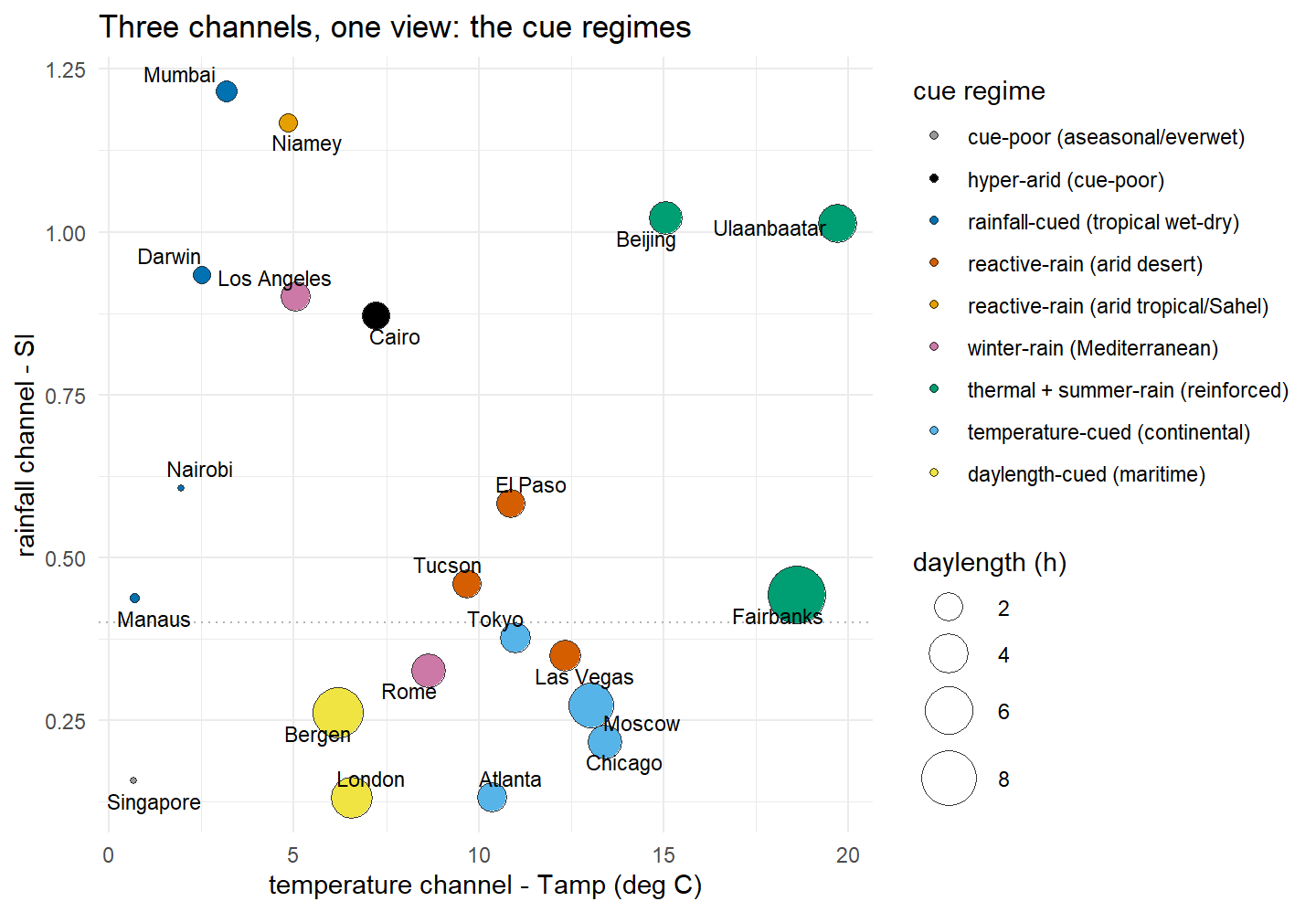
The whole scheme fits in one picture. Temperature seasonality runs along the bottom, rainfall seasonality up the side, and the size of each point is the daylength channel, so all three cues are present at once. Color is the regime the rule assigned.
Show the code
plot_regime_map(regimes) +labs(title ="Three channels, one view: the cue regimes")
The regimes occupy coherent territories. The cue-poor and maritime places sit low and left, where temperature and rainfall are both quiet, separated only by the daylength bubble size that tells London from Singapore. The deserts and the hyper-arid sit at moderate temperature and middling rain. The continental regimes run off to the right where the temperature channel is loud. The reinforced summer-rain cities ride high on both temperature and rainfall. The plot is busy because the world is, but the colors don’t scatter at random. Each regime holds its own ground, which is the first sign that the categories are tracking something real.
A scatter of twenty-one chosen cities is a promising start, not a proof. The cities were picked to be clear cases. The real test is whether the same rule, applied to every cell of a continent with no cities chosen in advance, still produces coherent regions rather than confetti. That is the question the maps answer, and it’s where the voyage has been heading all along.