4 Aridity Is Not Rainfall Total

Chapter 3 ended with a warning: the channels can be fooled, and the rainfall channel most of all. The rainfall seasonality index tells us how unevenly the rain is spread across the year, but it says nothing about whether there is enough rain to matter. A place can post a high seasonality on almost no rain at all. And the obvious repair, looking at the yearly total instead, turns out to fail in its own way. This chapter fixes the rainfall channel by measuring rain against the thing that consumes it, and the fix is a number we already met: the moisture balance.

Show the code

## --- Standard packages ---

## many useful functions (dplyr, ggplot2, readr, tibble, purrr, tidyr)
library(tidyverse)
## formatted tables
library(gt)

## --- Packages from github/kimbridges ---

## install once with: remotes::install_github("kimbridges/seasonalityr")
library(seasonalityr)

## --- Options and defaults ---

## suppress read_csv() column-type messages
options(readr.show_col_types = FALSE)

## data source, cited under every table
source <- "Monthly normals from WorldClim 2.1 (10 arc-minute), via seasonalityr."

## the 21-city index table (bundled; see Chapter 2 and the appendix)
idx <- read_csv("data/cities_indices.csv")

## a shared colour scale: rain phase, blue for winter, orange for summer
phase_fill <- scale_fill_gradient2(low = "#D55E00", mid = "#EEEEEE", high = "#0072B2",
                midpoint = 0.5, limits = c(0, 1), name = "cool-season rain")

4.1 The mirage in the index

Cairo gets about 26 millimeters of rain in a year, almost all of it in the cool months. Las Vegas, no one’s idea of a wet city, gets more than four times as much. Yet by the rainfall seasonality index Cairo looks far more seasonal than Las Vegas. The index is a ratio: it measures how concentrated the rain is, not how much there is. Concentrate almost nothing into a few months and the ratio climbs, even though those months hold a few millimeters between them. The seasonality is real arithmetic and an empty signal. Twenty-six millimeters in a year is not a wet season. It’s noise with a calendar.

So the rainfall channel needs a gate, something that asks not just when the rain falls but whether there is enough of it to be a cue at all. The first guess is the obvious one: use the yearly total. That guess fails too, and it’s worth seeing how.

4.2 The total is no fix

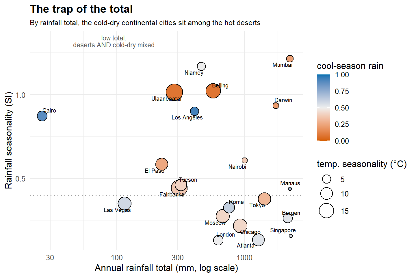
Lay the cities out by their rainfall total and their seasonality, and watch what happens at the dry end.

Show the code

ggplot(idx, aes(totP, SI)) +
  ## the low-total zone, where very different places pile up together
  annotate("rect", xmin = -Inf, xmax = 350, ymin = -Inf, ymax = Inf,
           fill = "grey85", alpha = 0.5) +
  annotate("text", x = 95, y = 1.32, size = 3, colour = "grey35", lineheight = 0.9,
           label = "low total:\ndeserts AND cold-dry mixed") +
  geom_hline(yintercept = 0.40, linetype = "dotted", colour = "grey60") +
  geom_point(aes(fill = cool_frac, size = Tamp), shape = 21, colour = "black") +
  ggrepel::geom_text_repel(aes(label = name), size = 2.7, max.overlaps = 20) +
  phase_fill +
  scale_size_area(max_size = 10, name = "temp. seasonality (°C)") +
  scale_x_log10() +
  labs(x = "Annual rainfall total (mm, log scale)", y = "Rainfall seasonality (SI)",
       title = "The trap of the total",
       subtitle = "By rainfall total, the cold-dry continental cities sit among the hot deserts") +
  theme_minimal(base_size = 12) +
  theme(plot.title = element_text(face = "bold"), plot.subtitle = element_text(size = 9.5))

The shaded band on the left is the low-rainfall zone, and it’s crowded with places that have nothing in common. The hot deserts are there, Las Vegas, Tucson, El Paso, Cairo. But so are Ulaanbaatar and Fairbanks, which are not deserts at all. They’re cold, dry, continental places where the modest rain that falls is plenty, because so little of it evaporates. Ulaanbaatar collects 282 millimeters; Tucson collects 318. By the total they’re twins. One is the Mongolian steppe under deep winter snow, the other a cactus desert. A cutoff drawn on rainfall total would have to call them the same.

Show the code

## five cities that break the rainfall-total test
idx |>
  filter(name %in% c("Cairo", "Las Vegas", "Tucson", "Ulaanbaatar", "Fairbanks")) |>
  arrange(totP) |>
  select(name, totP, SI, m_mean, Tamp) |>
  gt() |>
  fmt_number(columns = c(SI, m_mean, Tamp), decimals = 2) |>
  tab_header(title = "Same totals, different worlds") |>
  tab_footnote(footnote = "Annual rainfall, millimeters.",
               locations = cells_column_labels(columns = totP)) |>
  tab_footnote(footnote = "Water balance: mean monthly P - 2T. Negative is water-limited.",
               locations = cells_column_labels(columns = m_mean)) |>
  tab_footnote(footnote = "Temperature seasonality: half the annual range, °C.",
               locations = cells_column_labels(columns = Tamp)) |>
  tab_source_note(source_note = source)

name	totP¹	SI	m_mean²	Tamp³
Same totals, different worlds
Cairo	26	0.87	−41.03	7.21
Las Vegas	115	0.35	−29.89	12.33
Ulaanbaatar	282	1.01	26.38	19.70
Fairbanks	309	0.44	31.27	18.61
Tucson	318	0.46	−14.81	9.69
¹ Annual rainfall, millimeters.
² Water balance: mean monthly P - 2T. Negative is water-limited.
³ Temperature seasonality: half the annual range, °C.
Monthly normals from WorldClim 2.1 (10 arc-minute), via seasonalityr.

The column that pulls them apart is the last new one in the table, the water balance. Tucson’s is negative, Ulaanbaatar’s is positive, and that single sign is the difference between a desert and a cold steppe.

4.3 Rain against demand

The fix was in Chapter 2 all along. The moisture value m = P - 2T charges each month’s rain against twice its temperature, the rough stand-in for how much water the warm air takes back. Averaged across the year, m_mean is a place’s standing water balance: how the rainfall stacks up against the evaporative demand it has to meet. When it’s positive, the year ends in surplus and rain can be counted on. When it’s negative, demand wins and the place lives in deficit, however the rain is timed.

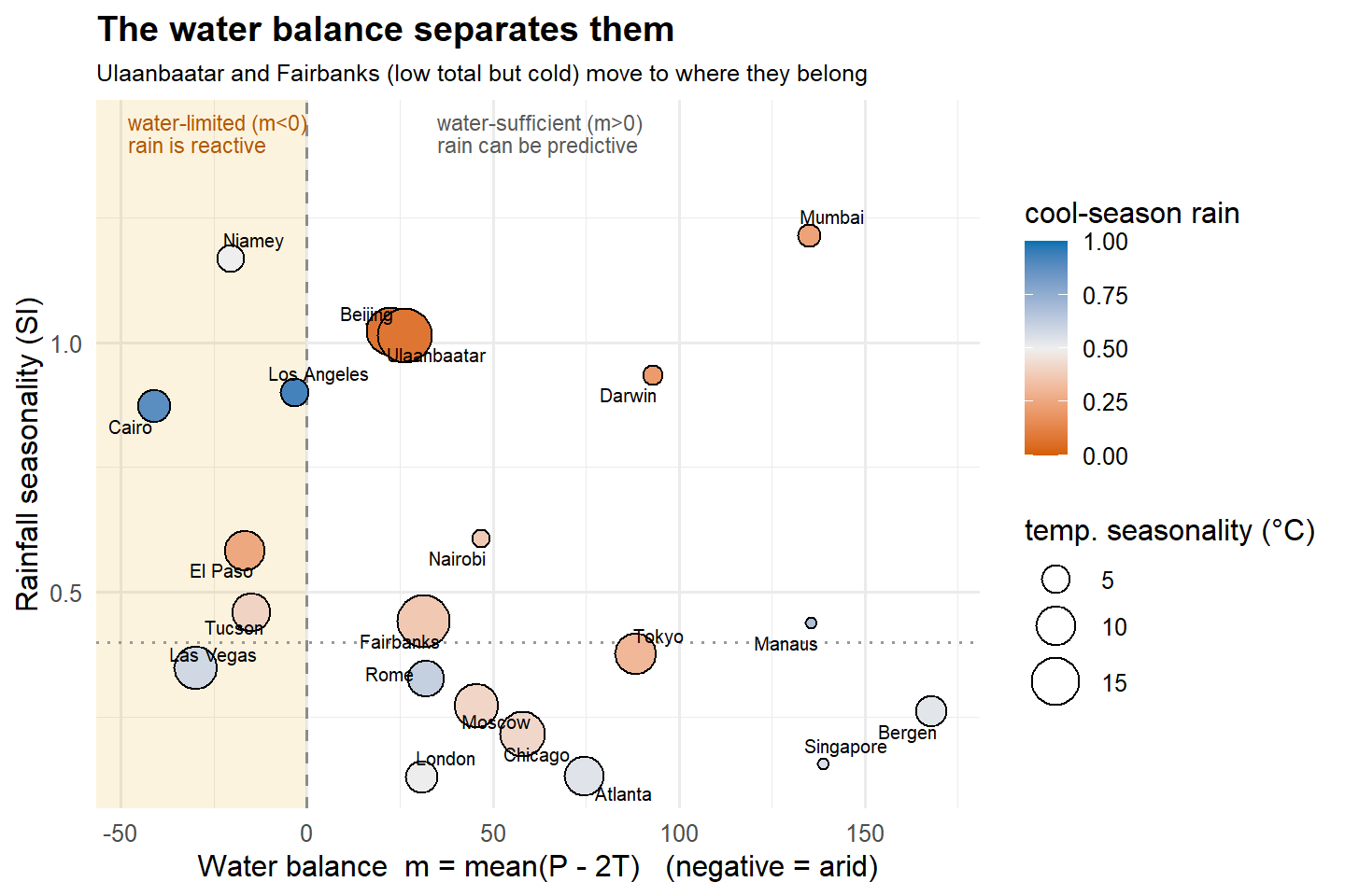
This is the true aridity axis, and it sorts the dry cities correctly where the total could not.

Show the code

ggplot(idx, aes(m_mean, SI)) +
  ## the water-limited side
  annotate("rect", xmin = -Inf, xmax = 0, ymin = -Inf, ymax = Inf,
           fill = "#E69F00", alpha = 0.13) +
  geom_vline(xintercept = 0, linetype = "dashed", colour = "grey55") +
  annotate("text", x = -48, y = 1.42, hjust = 0, size = 3, colour = "#B25900",
           lineheight = 0.9, label = "water-limited (m<0)\nrain is reactive") +
  annotate("text", x = 35, y = 1.42, hjust = 0, size = 3, colour = "grey35",
           lineheight = 0.9, label = "water-sufficient (m>0)\nrain can be predictive") +
  geom_hline(yintercept = 0.40, linetype = "dotted", colour = "grey60") +
  geom_point(aes(fill = cool_frac, size = Tamp), shape = 21, colour = "black") +
  ggrepel::geom_text_repel(aes(label = name), size = 2.7, max.overlaps = 20) +
  phase_fill +
  scale_size_area(max_size = 10, name = "temp. seasonality (°C)") +
  scale_x_continuous(expand = expansion(mult = c(0.04, 0.06))) +
  labs(x = "Water balance  m = mean(P - 2T)   (negative = arid)",
       y = "Rainfall seasonality (SI)",
       title = "The water balance separates them",
       subtitle = "Ulaanbaatar and Fairbanks (low total but cold) move to where they belong") +
  theme_minimal(base_size = 12) +
  theme(plot.title = element_text(face = "bold"), plot.subtitle = element_text(size = 9.5))

Now the dry cities fall on the correct sides of zero. Cairo sits deepest in deficit, the driest of them all, with its high seasonality index unmasked as the mirage it is. The hot deserts line up in the water-limited band beside it. And Ulaanbaatar and Fairbanks have crossed to the water-sufficient side, out among the temperate cities, exactly where a cold place whose rain meets its small demand belongs. Nothing about the rainfall changed. We just stopped counting millimeters and started weighing them against the heat.

4.4 Reactive and predictive rain

The sign of the water balance does more than label a place arid or not. It decides what kind of cue the rain can be, and that takes us back to the two kinds of cue from Chapter 1.

Where the balance is positive, rain is dependable enough to anticipate. A wet season arrives on a schedule a plant can prepare for, swelling buds before the rains rather than after. Rain there is a predictive cue, a clock. Where the balance is negative, there is no schedule to trust. The rain might come this month or next or not at all, and the only workable strategy is to wait and then move the moment the water arrives. Rain there is a reactive cue, a trigger. The desert plant that flowers within days of a storm and sleeps for years between is not keeping poor time. It’s keeping the only time its cue allows.

This is the gate the classifier in the next chapter will use. A place’s rainfall seasonality is taken at face value only when the water balance says the rain is real. Where the balance is negative, that same seasonality is read as a trigger, not a timetable, and where the rain is negligible against demand, the rainfall channel is switched off as a mirage. With temperature, daylength, and now a rainfall channel that knows when it’s telling the truth, we have the full set of cues. It’s time to assemble them into regimes.