1 The Two-Way Table
Before we come to the program or the package, we need the idea they serve. This chapter is about the two-way table itself: what it is, what makes it unusual among data structures, and why its particular way of looking for pattern is worth understanding. The ideas here are not specific to ecology, though ecology is where they were worked out. If you keep records of what occurs where, this chapter is about your data too.
1.1 A table of what occurs where
A two-way table records what occurs where. The rows are things that can occur. The columns are places they can occur in. A cell says whether — and sometimes how much — a given thing was found in a given place.
In vegetation ecology, the places are field samples called relevés. A relevé is a patch of ground a botanist has examined, listing every plant species in it. The things that occur are the species. Put a column for each relevé and a row for each species, and the table records which plants grew where. Often the cell holds a cover value — a rough measure of how much of the plot a species filled — but at its simplest a cell records only presence or absence.
Nothing about this structure is botanical. The rows are items and the columns are sites, and the pairing fits wherever items occur across sites. In ethnobotany, the sites might be traditional healers and the items the herbal species each one uses; the table then records which remedies are shared and which are particular, and it can be read to compare how different practitioners treat the same ailment. One could imagine comparing regional variations in a cuisine by treating menus as sites and dishes, or ingredients, as the items. The vocabulary changes with the field. The structure does not. For the rest of this document we use the vegetation vocabulary — relevés and species — because that is where the method was built. Keep the wider reach in mind as you read.
1.2 Mostly empty
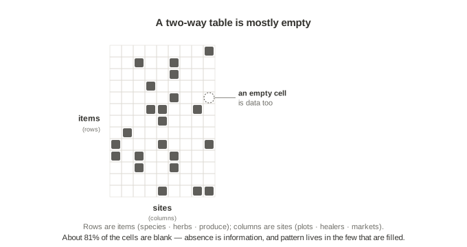
Here is the first thing that makes a two-way table unusual. It is mostly empty.
Most datasets are dense. A spreadsheet of patients, or transactions, or weather stations has a value in almost every cell, and a blank is treated as a problem — a missing value to be filled in, estimated, or dropped. A two-way table is the opposite. Any one relevé contains only a small fraction of all the species in the study, so most cells are blank. Blanks are the normal state, not the exception.
And the blanks carry meaning. That a species is absent from a relevé is a real observation, just as informative as its presence. When we look for pattern in a two-way table, we are reading the filled cells and the empty ones together. This is why the data are so often recorded as simple presence and absence: where a species occurs, and where it does not, is already most of the signal. The cover values add detail, but the bones of the pattern are in the geography of presence and absence.
1.3 Looking for pattern
What do we do with such a table? We look for pattern.
A raw two-way table, with its species and relevés in whatever order they were entered, shows nothing. The filled cells are scattered across it like static. The work is to sort it — to reorder the rows and the columns so that related species fall near each other and the relevés they favor line up beneath them. Done well, the scatter resolves into blocks: clusters of species that tend to occur together, sitting above the clusters of relevés where they occur. The table becomes legible. You can see, at a glance, that these species go with those sites.
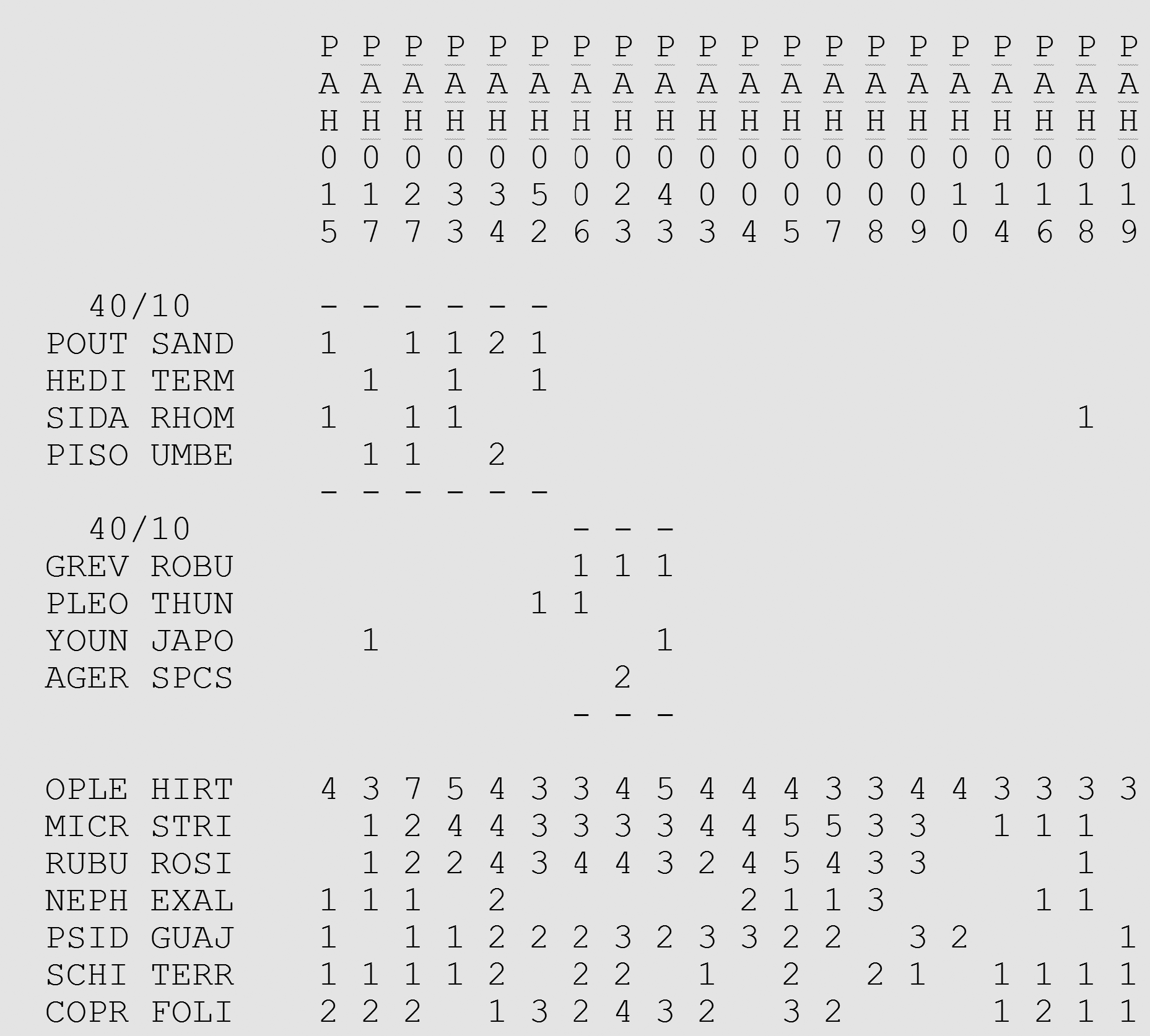
The figure above is such a table, sorted. It is one of the datasets we will use throughout this document: a forest survey from Hawai‘i. The dashes and the bracketed groups near the top are the pattern made visible. We will return to how that sorting is done. For now the point is only the goal: to turn an unreadable scatter into a picture you can read.
1.4 Setting aside the extremes
Now the part that can look strange. To find the pattern, we first throw away some of the data — on purpose, and at both ends.
Consider a species that occurs in almost every relevé. It is everywhere, so it tells us nothing about where. It cannot distinguish one group of sites from another, because it belongs to all of them. Now consider a species found in only one or two relevés out of many. It is too rare to mark a pattern; with so few occurrences there is no distribution to share with anything. Neither the ubiquitous species nor the rare one can help us sort the table.
So we set them aside. The very common species — the ones above a high threshold of occurrence — are pulled out and held apart. The very rare species — those below a low threshold — are pulled out too. The analysis then works only with the species in the middle: common enough to define a group, distinct enough to mark it. These are where pattern lives. The Braun-Blanquet tradition calls them the differential species; the coenosr package and most of this book call this kept middle band the eligible species. The two names emphasise different things — what the species do, and where they sit on the constancy scale — but they pick out the same set, and we will mostly say eligible from here on.
To someone trained to use all the data, discarding the most common and the rarest observations can seem backward. But it matches how people actually find pattern when they look. We notice the thing that is present here and absent there — the contrast. We do not learn much from what is everywhere, and we cannot learn much from what is almost nowhere. The method simply makes that instinct explicit, and applies it with a definite rule. Much of the rest of this document follows from this one decision, and the package carries it out in a single step.