Show the code
## data wrangling and formatted tables
library(tidyverse)
library(coenosr)The last chapters built the groups and admitted what they cost. This one asks the plain question that has waited underneath all of them: once you have the groups, what are they for? The two-way table you started with was deliberately impoverished. It threw away almost everything you know — a species became a name and a mark in a column, a site became a list of marks — and it did this on purpose, so that one kind of pattern could show through the clutter of everything else. The groups are where the discarded knowledge comes back. A group is a thing that did not exist in the raw data; it is a new unit, and almost everything you go on to do attaches to it.
## data wrangling and formatted tables
library(tidyverse)
library(coenosr)You always knew more than the table held. You know a species’ life form, whether it is a tree or a sedge or a vine; you know where each site sits, how high it is, what it grows on. The table left all of that out, not from ignorance but from discipline — the structure could only declare itself once the incidental detail was stripped away. Now that the groups are in hand, the detail can be joined back, one attribute at a time, to a group rather than to a scatter of separate sites.
Take the markets of the earlier chapters. Sorting separated them into two kinds by the produce they carried, and two markets that carried only staples sat in neither. Set against that grouping is everything we happen to know about the markets themselves — where each one is, how high it stands, how large it is — none of which went into the sort.
## the small market survey from the earlier chapters
rel <- read_lists("data/simple_10x15_simplified.txt")

## the site groups the sort produced. form_groups() returns, for each group,
## the species in it and the markets it occupies; we label the groups A, B, ...
## and mark the two markets that joined neither.
grp     <- form_groups(rel)
markets <- sort(as.integer(as.character(unique(rel$releve))))
members <- map_dfr(seq_along(grp),
                   \(i) tibble(market = as.integer(grp[[i]]$releves),
                               group  = LETTERS[i]))
groups <- tibble(market = markets) |>
  left_join(members, by = "market") |>
  mutate(group = replace_na(group, "—"))

## what we know about each market, beyond the produce it sells
info <- read_csv("data/market_info.csv", show_col_types = FALSE)groups |>
left_join(info, by = "market") |>
rename(`elevation (m)` = elevation_m)| market | group | district | elevation (m) | stalls |
|---|---|---|---|---|
| 1 | B | Uplands | 380 | 18 |
| 2 | A | Harbour | 12 | 24 |
| 3 | B | Uplands | 420 | 15 |
| 4 | A | Harbour | 8 | 22 |
| 5 | B | Uplands | 350 | 12 |
| 6 | A | Harbour | 15 | 26 |
| 7 | B | Uplands | 400 | 17 |
| 8 | A | Harbour | 10 | 25 |
| 9 | — | Crossroads | 120 | 6 |
| 10 | — | Crossroads | 95 | 7 |
Read the groups against the geography, and something quietly remarkable appears.
groups |>
  filter(group != "—") |>
  left_join(info, by = "market") |>
  group_by(group) |>
  summarise(markets               = n(),
            district              = paste(unique(district), collapse = ", "),
            `mean elevation (m)`  = round(mean(elevation_m)),
.groups = "drop")| group | markets | district | mean elevation (m) |
|---|---|---|---|
| A | 4 | Harbour | 11 |
| B | 4 | Uplands | 388 |
The two produce groups are also two places. One kind of market sits up in the hills, around four hundred metres; the other sits down by the harbour, near sea level. We never told the sort where the markets were. It found the division from the produce alone, and the geography agreed. That agreement is worth pausing on, and we return at the end of the chapter to why it carries the weight it does.
With the coordinates themselves the same join becomes a map: each site coloured by its group, the gaps between sampled sites filled by tessellation, so the groups read as regions rather than points. The phytosociologists who built this method rarely drew such maps, because filling the space between sparse relevés by hand was the labour of a career; a few managed it where air photographs gave them a guide. The computation that makes it routine arrived long after the method did. That map is a chapter of its own, and we leave it here as an invitation.
The simplest things you can do to a two-way table are to add up its rows and its columns, and both carry more than arithmetic. Adding along a row gives a species’ constancy, the number of sites it occupies, which is the very quantity that built the groups in the first place. Constancy is also the seed of a family of indices. In ethnobotany the same count, rephrased, becomes a measure of how widely a remedy is cited; the more practitioners who name a plant, the higher it scores. The Braun-Blanquet tradition has a word that bridges the two worlds: fidelity, a species faithful to one association, which is the same idea as a plant faithful to one use.
Here a question opens that is worth taking seriously. An index built from every row sum counts the ubiquitous staples and the lone rarities alongside everything else, and those are exactly the species the method set aside as carrying no signal. What if the index were built from the eligible species only, the discriminating middle the trim kept? The trim is the method’s own verdict about where the signal lives, and that verdict is reusable. The test to put to any index is simple: does it mean to discriminate, or to total? An index that wants to separate one group from another sharpens when the everywhere-and-nowhere species are dropped; an index that wants sheer magnitude, where being common is itself the point, wants them kept.
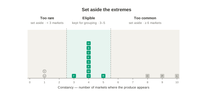
The column sums make the same case from the other direction.
## the eligible species are the middle band classify_species() keeps,
## set apart from the ubiquitous staples (L, C, P) and the rare items (U, Y)
eligible <- classify_species(rel) |>
  filter(status == "eligible") |>
  pull(species)

## total richness: items per market.  eligible richness: only the discriminating ones.
total_rich <- rel |>
  mutate(market = as.integer(as.character(releve))) |>
  count(market, name = "total richness")
ess_rich <- rel |>
  filter(species %in% eligible) |>
  mutate(market = as.integer(as.character(releve))) |>
  count(market, name = "eligible richness")

groups |>
  left_join(total_rich, by = "market") |>
  left_join(ess_rich,   by = "market") |>
mutate(`eligible richness` = replace_na(`eligible richness`, 0L))| market | group | total richness | eligible richness |
|---|---|---|---|
| 1 | B | 7 | 4 |
| 2 | A | 9 | 6 |
| 3 | B | 8 | 5 |
| 4 | A | 8 | 5 |
| 5 | B | 7 | 5 |
| 6 | A | 8 | 5 |
| 7 | B | 8 | 5 |
| 8 | A | 8 | 5 |
| 9 | — | 3 | 0 |
| 10 | — | 3 | 0 |
Adding down a column gives a site’s species number, its richness, and richness is the statistic most often mistaken for diversity, though the two are not the same. Counted across every item, the markets that sell only staples still score three; counted across the eligible species alone they score nothing, which is the truer reading, because what they lack is not produce but any produce that sets them apart. The grouped markets, by contrast, each carry most or all of their community’s five species — one market is missing a member, another has gained a sixth that strayed in from the other group — while the staple-only markets carry none. Had we recorded quantities rather than bare presence, we could compute a diversity index for each site as well, and the same question would return: the diversity of just the eligible species would measure not how varied a site is, but how varied its diagnostic signal is. That is a different number, honestly named, and often the more interesting one.
Every product in this chapter rests on the groups, and the groups, as the last chapter insisted, are drawn rather than found. So the map is an argument, and the index is an argument, and the eligible-species diversity is an argument, each inheriting whatever was provisional in the grouping beneath it. That sounds like a weakness until you see where it draws its line, and the line is the whole point.
There are two kinds of thing you can join to a group, and they answer to different rules. A statistic computed from the table itself — a constancy index, an eligible-species count — is conditioned on the very grouping it describes; it can illuminate the groups, but it cannot confirm them, because it was built from them. You cannot use the groups to prove the groups. The ancillary knowledge of the first half of this chapter is different in kind. The markets’ elevations and districts were never in the table; they are independent of it. When the produce groups line up with the hills and the harbour, that alignment is real evidence, precisely because it comes from outside. Independent data can corroborate a grouping; data derived from the grouping can only reason within it.
That distinction is why the whole enterprise counts as science rather than impression. The two-way table began as an intuition, a practised eye that saw, in a thicket of species and sites, that some belonged together. What the method added was not a better intuition but a reproducible one: the same rules, applied the same way, by anyone, leaving a record the next person can inspect and dispute. It does not prove that the groups are real. It makes of them an explicit, checkable argument, open to outside test and honest about its own conditioning. The groups are reproducible, not proven, and knowing the difference is what lets you trust them exactly as far as they have earned.