Show the code
## data wrangling and formatted tables
library(tidyverse)
library(coenosr)Every chapter so far has built toward a clean sorted table, as if a tidy answer were always waiting to be uncovered. Before the last technical matter, it is worth saying plainly what coenosr is for — because the answer is not always clean, and that is not a flaw.
coenosr looks for pattern in a two-way table. Pattern means several species that share a distribution, rising and falling together across the sites. Sometimes that pattern is sharp: distinct groups, each with its own block of sites, the diagonal staircase of the last chapter. Sometimes it is messy — groups that overlap, species that could belong to either, boundaries that blur. Sometimes there is no pattern at all, only scatter that no sorting will resolve, because the data hold none. Most real tables sit somewhere in between. The tool does not promise to find structure; it promises to look for it the same way every time, and to show you what it finds.
What makes that worth doing is the point of view. coenosr approaches a table from one deliberate stance: set aside the species too common or too rare to discriminate, then gather the rest into groups by whether they occur together inside a set of sites and stay away from the rest. That is the whole idea — a particular way of seeing, not the only way, but a clear one, and its clarity is its beauty.
And the search is not hidden. There is no statistical black box here, no optimisation to take on faith. The rules are simple enough to carry out by hand, with a pencil on a printed table — which is exactly what phytosociologists did for decades before COENOS, and exactly what Mueller-Dombois and Ellenberg set out step by step. COENOS automated the bookkeeping; it did not replace the reasoning. You can follow every move the program makes, because every move is a rule you could have made yourself.
## data wrangling and formatted tables
library(tidyverse)
library(coenosr)That openness lets us do something most software cannot invite: check the reconstruction against the original, group by group, and report exactly how close it came. Chapter 3 decoded the .S00 restart files COENOS left behind — the program’s own notes on how it sorted each table. Among those notes are the groups COENOS itself formed. We can treat them as an answer key.
## run coenosr on the Dieren data
rel    <- read_rel(system.file("extdata", "DIEREN.REL", package = "coenosr"))
groups <- form_groups(rel)

## COENOS's own groups, from the decoded .S00 oracle bundled with the package
orc <- read.csv(system.file("extdata", "dieren_s00_species.csv", package = "coenosr"),
                stringsAsFactors = FALSE)
orc$species <- trimws(orc$species)
coenos <- lapply(sort(unique(orc$role_code[orc$role_code > 0])),
                 \(g) orc$species[orc$role_code == g])

## for each coenosr group, find COENOS's most similar group and count shared species
comparison <- map_dfr(seq_along(groups), function(i) {
  found  <- groups[[i]]$species
  shared <- sapply(coenos, \(g) length(intersect(g, found)))
  best   <- which.max(shared)
  tibble(`coenosr group`   = i,
         `species found`   = length(found),
         `COENOS's group`  = length(coenos[[best]]),
         `shared`          = shared[best])
})comparison |>
transmute(`coenosr group`, `species found`,
`COENOS group size` = `COENOS's group`,
result = if_else(shared == `COENOS's group` & `species found` == `COENOS's group`,
"recovered exactly",
paste0(shared, " of ", `COENOS's group`, " recovered")))| coenosr group | species found | COENOS group size | result |
|---|---|---|---|
| 1 | 20 | 22 | 18 of 22 recovered |
| 2 | 13 | 18 | 11 of 18 recovered |
| 3 | 5 | 4 | 4 of 4 recovered |
Read down the last column. The small, well-separated group comes back whole — every species COENOS placed there, coenosr placed there too. The two larger groups come back close, eighteen of twenty-two and eleven of eighteen, differing only by a handful of species at their edges. The pattern in this table is itself the honest one: where the structure is sharp, the recovery is exact; where the structure is subtler, the recovery softens. The tool reports the data it was given, and Dieren’s data are real, not idealised — clear in places, blurred in others.
Those few species at the edges are where the recovery meets its limit, and it is worth being precise about what the limit is. When a species sits between two groups — occurring partly inside one and partly inside another — both groups have a claim on it, and something has to decide. COENOS decided by a tie-break: a rule for breaking ties among ambiguous species. That rule was never written down. It was not in the published method, not in the help file, and — we checked — not in the .S00 files either. The restart records preserved the seeds, the threshold levels, the iteration counts, and the relevé groups, but the quantities that would have driven the tie-break turned out to be merely the stored cover values, not the working statistics the program computed as it sorted. The decision lived only in the running code, and the running code is gone.
So the residual is sharp-edged and small: coenosr reproduces COENOS’s method, and reproduces its groups exactly wherever the groups are unambiguous, and parts company only on the species the original program had to make a judgement call about. A second, even finer detail goes the same way — the order among species of identical constancy within a group, a hand-sort nicety that left no trace to recover. Neither is a gap in the method. Both are private decisions of one particular program, lost when that program stopped running.
It is fitting that we can be this exact about what is missing, because being able to say precisely where a method is certain, close, or lost is the gift of a method with nothing hidden. A black box answers every question with the same confident single output and never tells you which parts it was sure of. An open one hands you the map.
There is a deeper symmetry here, and Mueller-Dombois and Ellenberg named it long ago. When Ceska and Roemer first ran their program on Ellenberg’s data, the two authors judged the result “a fairly close approximation of the hand-derived original.” COENOS was itself an approximation, one careful step away from the hand method it automated. coenosr is one more careful step from COENOS. At each step a little of the older craft is left behind, and at each step the loss is small and visible — visible precisely because none of these methods ever pretended to be an oracle. They were ways of looking, passed from a hand holding a pencil, to a program on a DOS machine, to an R package, each faithful to the last as far as the record allowed.
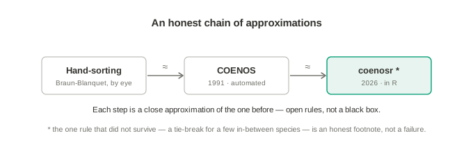
What survived the whole journey is not a binary file or a particular sorted table. It is the point of view: set aside the extremes, find the species that share a distribution, let the pattern declare itself. That way of seeing is legible again, runnable again, and — most of all — still simple enough to do by hand. The program died; the idea did not.