Everything so far has been about one forest. But the point of a tool is that it travels. If the method is any good, it should build a checklist for a place it has never seen — and the checklist it builds should tell that place’s own story, not a copy of Kīpuka Puaulu’s.
This chapter runs the same steps on a second site: the ʻIliau Loop, in the dry country above Waimea Canyon on Kauaʻi. Different island, different rainfall, different botanists, a different century of collecting. The two checklists share a family resemblance and disagree on almost everything else — and each disagreement is one of the earlier chapters, seen from a second angle.
Show the code
## --- Standard packages ---## data handling and graphics (dplyr, readr, ggplot2, ...)library(tidyverse)## formatted tableslibrary(gt)## spatial: the ʻIliau specimen maplibrary(sf)library(terra)library(tidyterra)## --- Package from github/kimbridges ---## install once with: install_github("kimbridges/checklistr")library(checklistr)## --- Options ---## suppress read_csv() column-type messagesoptions(readr.show_col_types =FALSE)
8.1 Same method, two floras
The same three lines of code that built the Kīpuka Puaulu checklist built the ʻIliau one; only the coordinates changed. Set the two results side by side.
Show the code
D <-"data/"ksp <-read_csv(paste0(D, "kipuka_puaulu_specimens_dedup.csv"))isp <-read_csv(paste0(D, "iliau_loop_specimens_dedup.csv"))kcl <-read_csv(paste0(D, "kipuka_puaulu_checklist_generated.csv"))icl <-read_csv(paste0(D, "iliau_loop_checklist_generated.csv"))## helper: the single most frequent value of a columntop1 <-function(x) names(sort(table(x), decreasing =TRUE))[1]compare <-tibble(Measure =c("Setting", "Taxa", "Records (deduplicated)", "Singletons","Collectors", "Leading collector", "Dominant herbaria","Determination conflicts", "Ferns (share of flora)"),`Kīpuka Puaulu (Hawaiʻi)`=c("mesic montane forest",nrow(kcl), nrow(ksp),sprintf("%d (%d%%)", sum(kcl$n_records ==1), round(100*mean(kcl$n_records ==1))),n_distinct(ksp$collector),paste0(top1(ksp$collector), " (1979–80 survey)"),"Bishop Museum (BISH/BPBM)",as.character(sum(kcl$det_conflict =="conflict", na.rm =TRUE)),sprintf("%d%%", round(100*mean(kcl$lifeform =="fern")))),`ʻIliau Loop (Kauaʻi)`=c("dry canyon-rim shrubland",nrow(icl), nrow(isp),sprintf("%d (%d%%)", sum(icl$n_records ==1), round(100*mean(icl$n_records ==1))),n_distinct(isp$collector),paste0(top1(isp$collector), " (modern, NTBG)"),"mainland (US, CAS, NY)",as.character(sum(icl$det_conflict =="conflict", na.rm =TRUE)),sprintf("%d%%", round(100*mean(icl$lifeform =="fern")))))compare |>gt() |>tab_source_note("Both checklists were generated by the same pipeline; only the query location differs.")
Measure
Kīpuka Puaulu (Hawaiʻi)
ʻIliau Loop (Kauaʻi)
Setting
mesic montane forest
dry canyon-rim shrubland
Taxa
160
44
Records (deduplicated)
167
62
Singletons
105 (66%)
32 (73%)
Collectors
29
20
Leading collector
Cuddihy (1979–80 survey)
Wood (modern, NTBG)
Dominant herbaria
Bishop Museum (BISH/BPBM)
mainland (US, CAS, NY)
Determination conflicts
8
0
Ferns (share of flora)
21%
11%
Both checklists were generated by the same pipeline; only the query location differs.
The two floras are the same kind of object built the same way, and almost every row differs — not randomly, but along the exact seams the earlier chapters exposed.
8.2 The same threads, seen twice
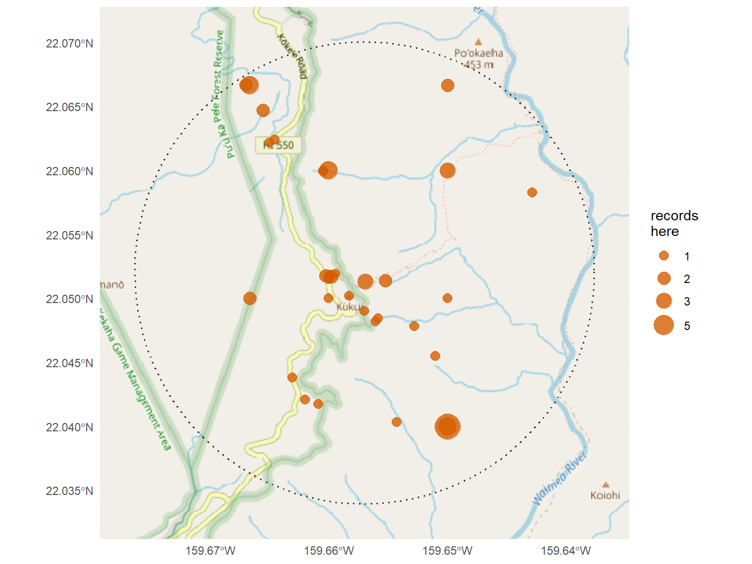
Scale and the map. Kīpuka Puaulu’s records stack on a handful of named localities — the collecting habit and the gazetteer, made visible in Chapter 3. ʻIliau’s do not: its 62 records fall on 35 distinct coordinates, scattered along the loop. The difference is an era. ʻIliau was worked recently, with a GPS in hand, so each collection carries its own true position; Kīpuka’s older sheets were placed by name after the fact. The same map that revealed taxonomic stacking on one island reveals modern point-sampling on the other.
Show the code
## ʻIliau specimen locations, sized by records at each pointiliau <-read_csv("data/iliau_loop_specimens_dedup.csv") |>filter(!is.na(decimalLatitude), !is.na(decimalLongitude))ilocs <- iliau |>count(decimalLongitude, decimalLatitude, name ="n_records")ilocs_sf <-st_as_sf(ilocs, coords =c("decimalLongitude", "decimalLatitude"), crs =4326)## 2 km query circle around the trail (Kauaʻi = UTM 4N)icircle <-st_sfc(st_point(c(-159.657, 22.052)), crs =4326) |>st_transform(32604) |>st_buffer(2000) |>st_transform(4326)## cached street basemap (saved so the page renders offline)ibase <-rast("data/iliau_basemap.tif")ie <-ext(ibase)ggplot() +geom_spatraster_rgb(data = ibase, maxcell =Inf) +geom_sf(data = icircle, fill =NA, color ="grey20", linetype ="dotted", linewidth =0.7) +geom_sf(data = ilocs_sf, aes(size = n_records), color ="#D55E00", alpha =0.8) +scale_size_area(max_size =9, breaks =c(1, 2, 3, 5)) +coord_sf(xlim =c(ie[1], ie[2]), ylim =c(ie[3], ie[4]), expand =FALSE) +labs(size ="records\nhere") +theme_minimal(base_size =11) +theme(axis.title =element_blank())
ʻIliau Loop records on a street basemap, sized by records per location; the dotted line is the two-kilometre query area. Compare with the Kīpuka Puaulu map of Chapter 3: instead of a few heavy stacks on named localities, the points scatter along the trail and canyon rim — each a GPS-placed field collection.
Conflict and the institution. Kīpuka Puaulu had eight determination conflicts; ʻIliau has none. This is not because Kauaʻi’s botanists were more careful. It is because Kīpuka’s specimens are Bishop Museum sheets, double-entered under two institution codes — the very mechanism of Chapter 5 — while ʻIliau’s are held by mainland herbaria that reach GBIF by a single path. No double-entry, no self-contradiction. The conflict count is a fingerprint of where the specimens live, not of how well they were named.
Growth form and climate. Ferns are 21% of the mesic Kīpuka flora but only 11% at dry ʻIliau — the ecological signal Chapter 6 promised, read straight off two checklists. Ferns need humidity to reproduce; a drier site has fewer of them. The growth-form field, coarse as it is, carries enough information to separate a moist forest from a dry shrubland without a single field visit.
Collectors and the century. Each list is dominated by one collector, but from opposite ends of the record. Kīpuka’s is Cuddihy’s 1979–80 survey — a single historical campaign. ʻIliau’s is modern work by Ken Wood of the National Tropical Botanical Garden. Which brings the previous chapter’s point home in the most concrete way: the ʻIliau checklist exists at all because NTBG’s Kauaʻi collections are in GBIF. A specialty herbarium’s decision to contribute is why a reader can build this second flora — and why the comparison in this chapter is possible.
8.3 What travels, and what doesn’t
The method travels; the flora does not. The pipeline made no assumptions about Hawaiʻi, mesic forest, or Bishop Museum — hand it a different point and it returns a different place’s story, told in that place’s own records. What does not transfer is any single site’s character: ʻIliau is not a smaller Kīpuka, and a checklist that pretended otherwise would be lying. The value of a second site is exactly that it holds the first one’s peculiarities up to the light. One forest teaches you the tool. Two forests teach you which of your findings were about the method and which were about the place.