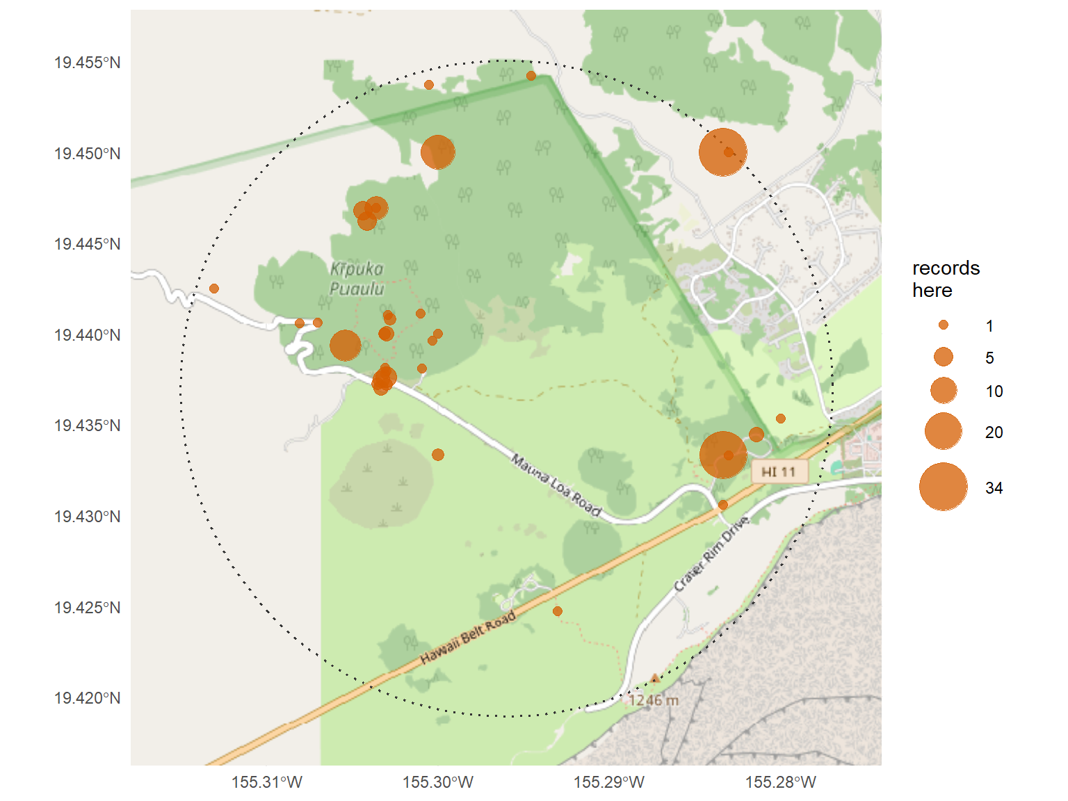
I know this forest, so when I first mapped its records I could read the map the way you read a familiar street. Inside the two-kilometre circle I had drawn, the points were not scattered evenly. A tighter cluster hugged the loop trail through the kīpuka itself, where I had walked so many times — and then a few heavy clumps sat off on their own, out by the roads. One of those clumps I can place exactly: a spot on Highway 11 I still slow down for, because it is one of the few places I know to see a particular uncommon plant. The map was not showing me where the plants grow. It was showing me where botanists had recorded them — and those are not the same thing.
That gap is the subject of this chapter. It is the quiet fact that governs everything the checklist can and cannot tell you.
Show the code
## --- Standard packages ---## data handling and graphics (dplyr, readr, ggplot2, ...)library(tidyverse)## formatted tableslibrary(gt)## --- Spatial packages (for the specimen map) ---## vector geometry (points, the query circle)library(sf)## raster handling (the cached street basemap)library(terra)## draw a SpatRaster basemap inside ggplotlibrary(tidyterra)## --- Package from github/kimbridges ---## install once with: install_github("kimbridges/checklistr")library(checklistr)## --- Options ---## suppress read_csv() column-type messagesoptions(readr.show_col_types =FALSE)
3.1 Two ways to collect a plant
There are two reasons to gather a plant and press it, and they lead to two very different maps.
The first reason is ecological: you want to know what grows where, and in what abundance. So you sample places. Every plot, every stop along a transect, earns its own collection — and collecting a species you already have is not waste, it is a data point. Do this and the specimens spread across the landscape, because the landscape is the thing being measured.
The second reason is taxonomic: you want to know what species exist in a region. Here one good sheet per species is enough. A collector who knows the herbarium already holds a Kīpuka Metrosideros does not press another; she moves on to something not yet represented. Do this and the specimens do not map the landscape at all. They map a checklist — one representative per taxon — pinned to whatever localities were convenient.
The herbarium record is built overwhelmingly on the second logic. This is not a defect; it is what herbaria are for. But it means that when we draw a circle on a map and call the result a flora, we are reading a taxonomic accumulation as though it were an ecological survey. The map remembers the difference even when we forget it.
3.2 What the map shows
The basemap comes from OpenStreetMap, retrieved once with the maptiles package and cached alongside the data so this page renders without the network.
Show the code
## fetch a street basemap for the query area (done once, then cached)library(maptiles)basemap <-get_tiles(x = circle,provider ="OpenStreetMap",zoom =14,crop =TRUE)
Each specimen carries a latitude and longitude. Collapsing the records to their distinct locations, and sizing each point by how many records sit on it, turns the collecting habit into something you can see.
Show the code
## specimen locations: one point per distinct coordinate, sized by records theregeo <-read_csv("data/kipuka_puaulu_specimens_geo.csv") |>filter(!is.na(decimalLatitude), !is.na(decimalLongitude))locs <- geo |>count(decimalLongitude, decimalLatitude, name ="n_records")locs_sf <-st_as_sf(locs, coords =c("decimalLongitude", "decimalLatitude"),crs =4326)## the 2 km query circle around the documented search centercircle <-st_sfc(st_point(c(-155.296, 19.437)), crs =4326) |>st_transform(32605) |># UTM 5N, so the buffer is in metresst_buffer(2000) |>st_transform(4326)## the cached street basemap (saved so the page renders offline)basemap <-rast("data/kipuka_basemap.tif")e <-ext(basemap)ggplot() +geom_spatraster_rgb(data = basemap, maxcell =Inf) +geom_sf(data = circle, fill =NA, color ="grey20",linetype ="dotted", linewidth =0.7) +geom_sf(data = locs_sf, aes(size = n_records),color ="#D55E00", alpha =0.75) +scale_size_area(max_size =12, breaks =c(1, 5, 10, 20, 34)) +coord_sf(xlim =c(e[1], e[2]), ylim =c(e[3], e[4]), expand =FALSE) +labs(size ="records\nhere") +theme_minimal(base_size =11) +theme(axis.title =element_blank())
Herbarium records for the two-kilometre circle around Kīpuka Puaulu, on a street basemap. Points are distinct collecting locations, sized by the number of records at each; the dotted line is the query radius. Streets give the eye a distance reference: Highway 11, Mauna Loa Road, Crater Rim Drive.
The arithmetic is stark. 164 georeferenced records fall on just 36 distinct locations. Half of those locations hold a single record, while one location alone absorbs 34. If the collecting had been ecological — a plant pressed at each place it was found — the points would disperse across the forest. Instead they pile up: a tight knot along the trail, where the intensive surveys worked, and a handful of dense stacks out by the roads, where records were pinned to a named place rather than a found one.
3.3 The georeferencing caveat
There is a second cause tangled into the same picture, and honesty requires separating it from the first. Most of these coordinates were not recorded in the field. Older sheets carry a written locality — “Kīpuka Puaulu,” “Kīpuka Ki,” “along the Mauna Loa road” — and a coordinate was attached later, by looking that place name up in a gazetteer. Every record that names the same locality then lands on the same point, whether or not the plants stood together. So some of the stacking is a collecting habit made visible, and some of it is a georeferencing method made visible. Both push the points toward named localities and away from an even scatter, but they are different phenomena: one is about how botanists collected, the other about how their labels were later turned into numbers. Whenever people speak of “recovering” old records, this is the seam they are working along, and it is worth naming rather than smoothing over.
3.4 Why a two-kilometre circle is not a plot
Put the two together and the checklist’s true scale comes into focus. It is not a census of a point on the ground; it is a taxonomic accumulation over a region — an honest record of which species have been collected somewhere within reach of this trail, over more than a century, by people who mostly did not need to collect any species twice. That is a real and useful thing. It answers “what grows in this area?” well. It is nearly silent, though, on the questions an ecologist would ask next: how common is each species, where exactly does it grow, what grows beside it. The circle sets the boundary of the search. It does not make the search a survey.
3.5 What this governs
Almost every caution in the chapters that follow descends from this one idea. When we ask how complete the checklist is, the estimators will assume ecological sampling — that a species seen once was seen once by chance — and the taxonomic habit will quietly break that assumption, because here a species is often collected once on purpose. The singletons that follow are not all signs of undersampling; many are the collecting logic showing through. Scale is the lens; the next chapter holds the count up to it.